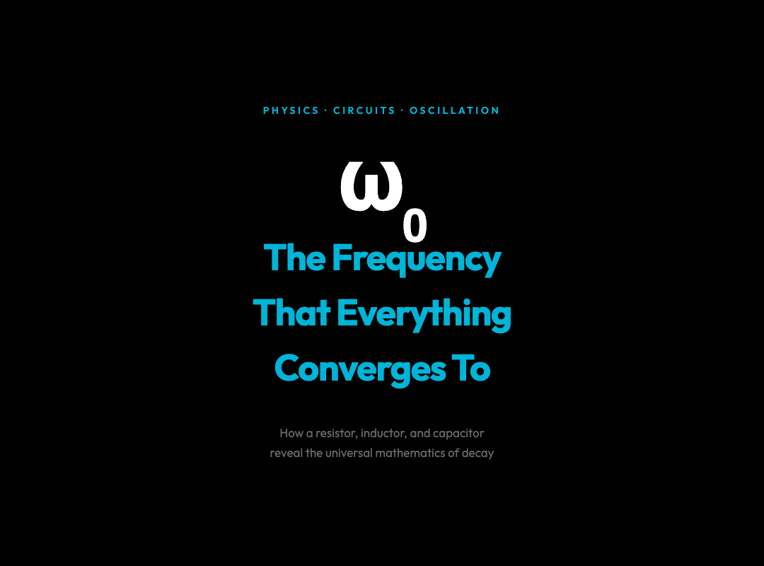
The Spiral That Appears Everywhere: What a Simple Circuit Reveals About the Nature of Decay
Charge a capacitor. Connect it to an inductor. Watch the voltage across the circuit swing wildly at first, then quieter, then quieter still — until it stops. You’ve just watched energy die in slow motion, expressed in the language of differential equations and spiraling phase trajectories.
The RLC circuit — a resistor, an inductor, and a capacitor wired in series — is one of the most teaching-dense systems in all of physics. Its behavior is governed by one equation:
Lq” + Rq’ + q/C = 0
Three terms. One for inertia (the inductor resists changes in current), one for dissipation (the resistor converts electrical energy to heat), and one for restoration (the capacitor pushes charge back toward equilibrium). From this single equation flows an entire taxonomy of behavior: underdamped oscillation, critical damping, overdamped decay, and resonance.
Each of these behaviors appears elsewhere in nature, and the connections are not merely metaphorical.
The Underdamped Case: When Oscillation Outlives Itself
Set the resistance low. The circuit rings — charge sloshing back and forth between capacitor and inductor, current leading voltage by a quarter cycle. The frequency of this damped oscillation is:
ω_d = √(ω₀² − γ²)
where ω₀ = 1/√(LC) is the natural frequency and γ = R/2L is the damping coefficient. The amplitude decays as e^(−γt), while the frequency is slightly below the ideal case.
What makes this interesting is not the circuit — it’s that the same equation describes a pendulum swinging underwater, a cavity laser losing photons, a population overshooting its carrying capacity, and a stock price briefly spiking before returning to fundamental value. The underdamped harmonic oscillator is a universal motif, and the RLC circuit lets you see every parameter, adjust it in real time, and watch the transition between regimes.
The Phase Portrait: A Spiral Is a Spiral Is a Spiral
The most revealing view of an RLC circuit is not voltage versus time. It is the phase portrait — charge on the x-axis, current on the y-axis.
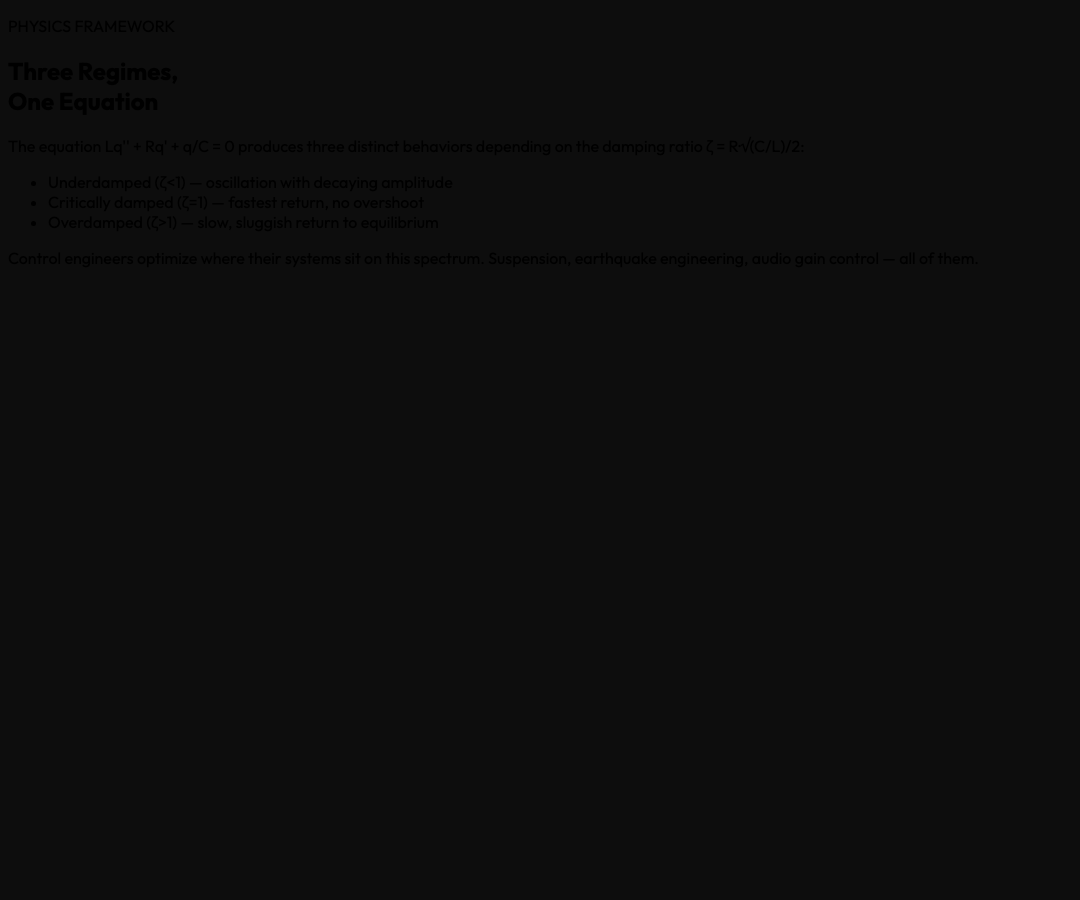
In an ideal LC circuit (no resistance), the trajectory is a closed ellipse, tracing constant energy. Add resistance and the ellipse becomes a spiral, curling inward toward the origin as energy bleeds away as heat. Each full loop represents one oscillation cycle. The tighter the spiral, the greater the damping.
This same spiral geometry appears in:
– Predator-prey models in ecology (Lotka-Volterra), where populations spiral toward equilibrium – The arms race between competing technologies, where advantages decay as heat (dissipation) removes them – Opinion dynamics in social systems, where controversial views gradually moderate toward consensus
The phase portrait strips away the calendar and shows you only the geometry of change. Two systems that share the same phase structure — the same topological features, the same inward spiral — are operating by the same underlying logic, regardless of whether they involve electrons, foxes, or financial speculators.
Resonance: When Forcing Finds the Natural Frequency
Apply an alternating voltage source to the circuit and drive it. The steady-state current amplitude depends on drive frequency ω according to:
I = V / √(R² + (ωL − 1/ωC)²)
At ω = ω₀ = 1/√(LC), the inductive and capacitive reactances cancel. Current reaches its maximum. This is resonance — and the sharpness of the peak is measured by the quality factor Q = ω₀L/R.
High-Q circuits (low resistance relative to reactance) have very sharp resonance peaks. This is how a radio tuner picks a single station from the air: the station’s carrier frequency hits the circuit’s natural frequency, current spikes, and the signal is extracted from noise.
The physics is identical to a swing. Push a swing at its natural frequency and it builds amplitude with each push. Push at the wrong frequency and the swing barely moves. The mathematics is the same. The RLC circuit is, again, the same phenomenon in electrical clothing.
Damping Regimes as a Decision Framework
Here is where the circuit becomes useful beyond physics.
The three damping regimes map directly onto how systems respond to displacement from equilibrium:
| Regime | Behavior | ———– | |
|---|---|---|---|
| ———- | Underdamped (ζ < 1) | Most common in nature | |
| Fastest return, no oscillation | Respond quickly, don’t overshoot | Overdamped (ζ > 1) | Systems with heavy friction |
Control engineers spend careers optimizing where a system sits on this spectrum. Too underdamped and a control system oscillates and overshoots (the Mars Climate Orbiter, the Boeing 737 Max). Too overdamped and it can’t respond fast enough to disturbances. The sweet spot — critical damping — is a design target for suspension systems, earthquake engineering, and automatic gain control in audio.
The RLC circuit lets you place any system at any point on this spectrum and watch the consequences in real time. That is not a small thing.
Energy: Where It Goes and Why It Never Comes Back
The circuit’s total energy at any moment is:
E = q²/2C + LI²/2
The first term is energy stored in the capacitor’s electric field. The second is energy stored in the inductor’s magnetic field. In an ideal LC circuit, these trade off perfectly — when one is maximum, the other is zero — and total energy is constant.
The resistor breaks this symmetry. At every instant, power P = I²R is being converted to heat and lost irretrievably. The total energy decays as:
E(t) = E₀ · e^(−2γt)
This is the Second Law of Thermodynamics in miniature. The RLC circuit is an entropy pump: it takes ordered energy (coherent oscillation) and converts it to disordered energy (heat). The spiral in the phase portrait is the signature of this process — a system with a memory of its initial condition gradually forgetting it, as information is erased into thermal noise.
This is also the mathematics of forgetting, of radioactive decay, of any process described by exponential decay. The circuit is not an analogy. It is the same mathematics, implemented in copper and glass.
Try It Yourself
The RLC Circuit Oscillation interactive visualization lets you manipulate resistance, inductance, and capacitance with sliders, and switch between waveform view, phase portrait, frequency response, and energy tracking — all in real time.
Set R to zero and watch the ellipse become a closed orbit. Crank R up past the critical value and watch the system become sluggish and overdamped. Drive the circuit at varying frequencies and watch the resonance peak emerge in the frequency response plot. It is the complete physics of damping, oscillation, and resonance in a single interactive page.
The Circuit as a Mirror
The RLC circuit is deceptively simple. Three components. One second-order differential equation. And yet it is a mirror held up to phenomena across science: population dynamics, economic adjustment, ecological succession, neutron stars, and laser cavities all share its essential structure.
When you understand why the spiral always curls inward — why the energy always drains — you understand something about the direction of time itself. The RLC circuit is, at its core, a machine for watching entropy increase.
That is remarkable for a handful of components you can hold in your hand.