The Duffing oscillator is a reminder that simplicity and complexity are not opposites. One clean equation — ÿ + δẏ + αy + βy³ = γ cos(ωt) — produces phase portraits that look like entire galaxies, Poincaré sections that reveal fractal structure, and windows of perfect periodicity that dissolve into chaos the moment you nudge a single parameter. This is not a flaw of physics. It is the physics. The world does not switch between “predictable” and “chaotic.” It moves along a spectrum, and the Duffing equation is one of the clearest windows onto that spectrum we have ever built.
The first time I ran the interactive Duffing oscillator visualization with default settings, I expected the chart to settle into a neat repeating pattern. It did not. The phase portrait spiraled and folded in on itself without ever repeating — a trajectory that traced out a shape with no edges and no resolution, the mathematical equivalent of a coastline seen from orbit.
What I was looking at was chaos. Not randomness — chaos is deterministic. The same starting conditions always produce the same trajectory. But the trajectory never repeats, and tiny differences in where you start multiply until the long-term behavior becomes genuinely impossible to forecast. This is not a computer glitch. It is the Duffing oscillator doing exactly what it is supposed to do.
One Equation, Three Regimes
The Duffing equation describes the motion of a nonlinear spring — one whose restoring force does not scale linearly with displacement. Where a simple harmonic oscillator follows F = −kx (Hooke’s law), the Duffing system adds a cubic term:
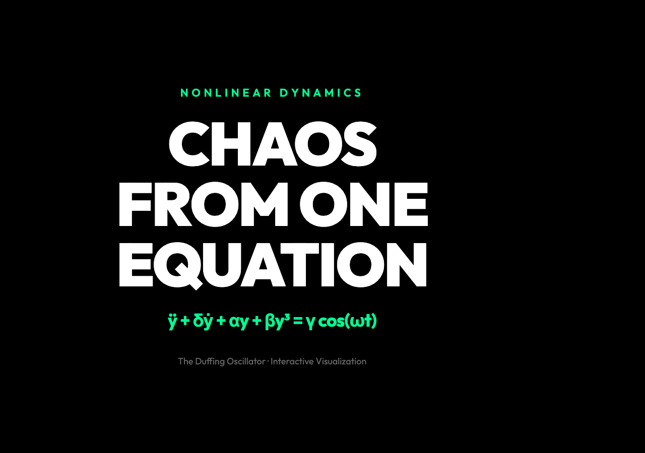
ÿ + δẏ + αy + βy³ = γ cos(ωt)
Each parameter controls a different dimension of the system’s behavior. The damping coefficient δ bleeds energy out of the system over time. The linear coefficient α determines whether the spring is hardening or softening — positive α gives a single stable equilibrium, negative α creates a double-well potential with two stable positions. The nonlinear coefficient β scales the cubic term. And γ cos(ωt) is a periodic driving force that continuously pumps energy back in.
Change γ, the drive amplitude, and the system crosses between three fundamentally different regimes: periodic (the system settles into a repeating pattern), chaotic (long-term trajectories become sensitive to initial conditions), and back to periodic again. The transitions are not gradual. They happen suddenly, at precise parameter thresholds that can be calculated but never eliminated.
This bifurcation structure is why the Duffing oscillator has been studied in engineering, physics, and mathematics for over a century. It is the simplest mechanical system that genuinely exhibits chaos.
What the Phase Portrait Shows
The phase portrait is the most intuitive window into the Duffing oscillator’s behavior. Plot position on one axis and velocity on the other, and each point represents a complete state of the system at one instant. As time evolves, the system traces a curve.

In the periodic regime, that curve closes on itself — the system returns to the same state after every driving cycle, and the phase portrait is a clean limit cycle. In the chaotic regime, the trajectory never closes. It fills a region of the phase plane without ever crossing itself, creating the kind of intricate, self-similar structure that mathematicians call a strange attractor.
The strange attractor is not a pattern the system is trying to repeat. It is the fingerprint of deterministic chaos — a shape that has structure at every scale, that emerges from the equations without any randomness, and that cannot be reduced to a simpler description.
Poincaré Sections: Slicing Through Chaos
A Poincaré section is a snapshot of the system’s state taken once per driving cycle. If the motion is periodic, every snapshot lands on the same point. The section is sparse and clean. If the motion is chaotic, the snapshots land on different points each cycle — but they cluster along a curve that reveals the attractor’s geometry.

This is where fractal structure appears. Zoom into a Poincaré section of a chaotic Duffing trajectory and you find that the apparently solid curve is actually a collection of thin, folded bands. Zoom into one of those bands and you find more bands, folded again. The self-similarity is not approximate — it is exact at every scale, a hallmark of fractal geometry that connects the Duffing oscillator to topics as distant as coastline measurement and market price charts.
The Poincaré section is also a practical diagnostic tool. By plotting where the system lands each cycle, you can distinguish periodic from quasi-periodic from chaotic motion at a glance, even when the time-domain trace looks complicated.
Potential Energy: Why the Double-Well Matters
The Duffing oscillator’s potential energy function is what makes it interesting. For α < 0, the potential has two wells:
V(y) = −0.5αy² + 0.25βy⁴
Visualize this and you see two valleys separated by a hill. A particle in this potential can rest in either valley — two stable equilibria. But if you drive it hard enough, the particle can climb over the barrier and jump between wells.
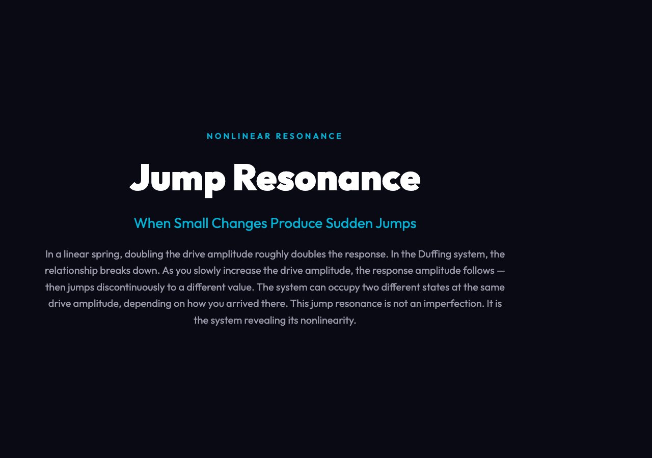
This is where the interesting nonlinear effects appear. In a linear spring, doubling the drive amplitude roughly doubles the response amplitude. In the Duffing system, small changes in drive amplitude can cause the response to jump discontinuously between two possible amplitudes — a phenomenon called jump resonance. This is not a theoretical curiosity. Engineers designing filters, bridges, and microelectromechanical systems have to account for it because it can cause sudden, catastrophic amplitude swings in real structures.
Butterfly Effect, Local and Global
The Duffing oscillator’s sensitivity to initial conditions is the feature that makes it chaotic. But there are actually two kinds of sensitivity worth distinguishing.
Local sensitivity — the butterfly effect — is exponential amplification of arbitrarily small differences in starting conditions. Two trajectories that start one micrometer apart will diverge exponentially, so that after a moderate time horizon, their paths have nothing to do with each other. This is why long-term weather prediction fails. It is also why the Duffing oscillator’s long-term future is unknowable even though its dynamics are fully deterministic.
Global sensitivity is subtler. In many chaotic systems, including the Duffing oscillator, the chaotic region of parameter space is not uniformly chaotic. Interspersed with the chaotic zones are periodic windows — parameter ranges where the motion stabilizes. The transition between chaos and periodicity is abrupt and often involves period-doubling bifurcations: the system moves from period-1 to period-2 to period-4 as a parameter changes, then cascades into chaos through an infinite sequence of period-doublings in a ratio that converges to the Feigenbaum constant δ ≈ 4.6692…
This universality is one of the most beautiful results in nonlinear dynamics. The same Feigenbaum constant describes period-doubling cascades in completely different systems — the Duffing oscillator, the logistic map, fluid convection, and lasers. This is not coincidence. It is a fingerprint of a deeper mathematical structure that the Duffing equation shares with a remarkable family of nonlinear systems.
What You Can Change and What You Cannot
The interactive visualization exposes five parameters directly: damping δ, linear coefficient α, nonlinear coefficient β, drive amplitude γ, and drive frequency ω. These are the levers available to you as an experimenter. And they are remarkably powerful.
Set δ = 0.1, α = −1.0, β = 1.0, γ = 0.0, ω = 0.0 and you have a free, undamped oscillator in a double-well potential. Add a small drive (γ = 0.3) and the system begins to oscillate in one well. Increase the drive to γ = 0.5 and the trajectory can suddenly cross the barrier, jumping between wells in a pattern that never stabilizes. Push further into the chaotic regime and the phase portrait blooms into its full strange-attractor complexity.
None of these regimes is more “correct” than the others. They are all embedded in the same equation. The parameter space of the Duffing oscillator is a complete physical universe — one that contains periodicity, chaos, bifurcations, and fractal structure in a single mathematical object you can fit on a desk.
The Duffing oscillator is a reminder that simplicity and complexity are not opposites. One clean equation — ÿ + δẏ + αy + βy³ = γ cos(ωt) — produces phase portraits that look like entire galaxies, Poincaré sections that reveal fractal structure, and windows of perfect periodicity that dissolve into chaos the moment you nudge a single parameter. This is not a flaw of physics. It is the physics. The world does not switch between “predictable” and “chaotic.” It moves along a spectrum, and the Duffing equation is one of the clearest windows onto that spectrum we have ever built.