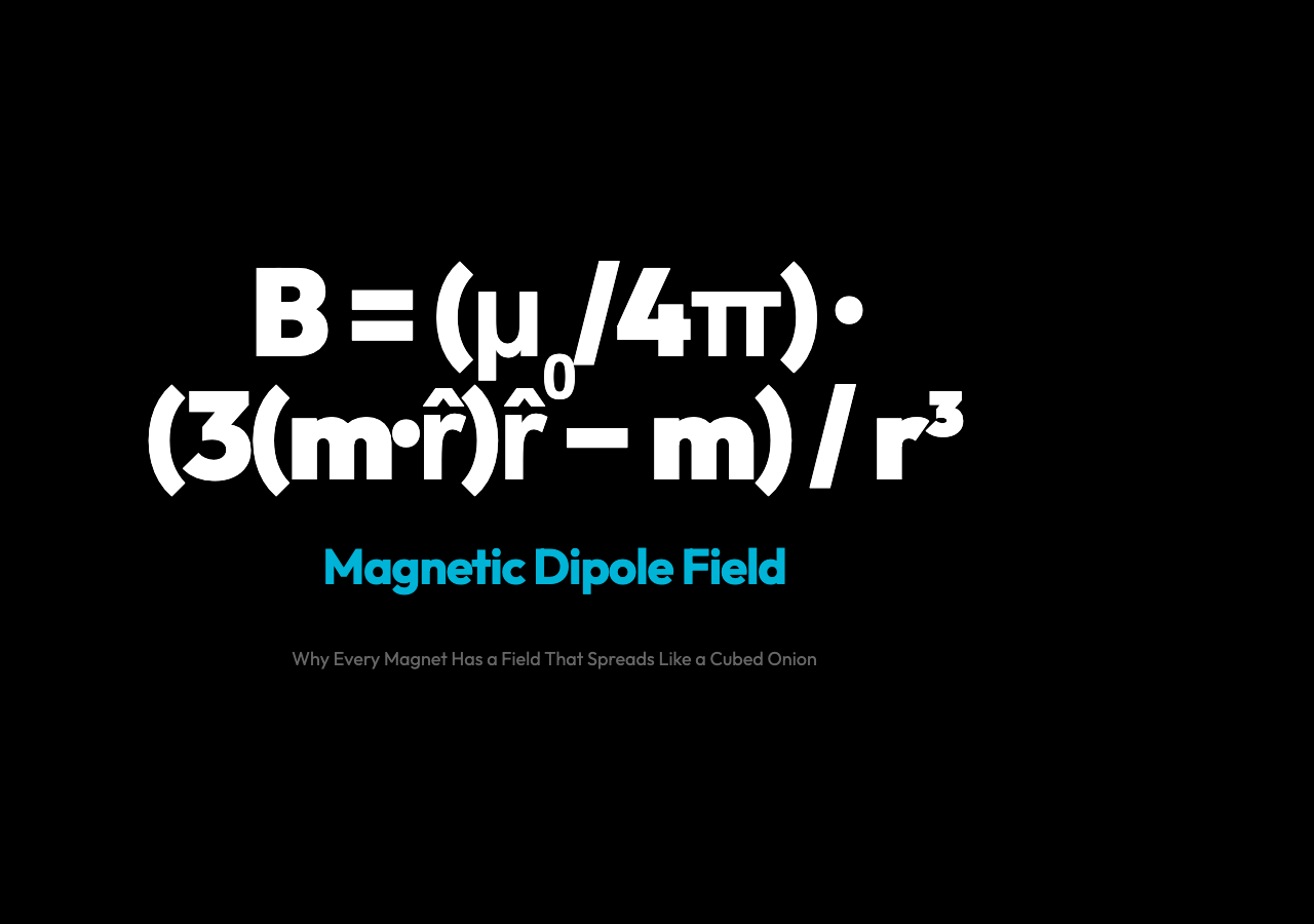
The bar magnet on your desk is surrounded by an invisible geometry that extends infinitely in all directions — and that geometry follows one of the cleanest equations in physics. Every point in space around the magnet has a magnetic field vector B pointing in a specific direction with a specific strength. If you could see the field lines, they would emerge from the north pole, arc gracefully through space, and re-enter the south pole. No two lines ever cross. That is not a approximation — it is a mathematical necessity.
The magnetic dipole field visualization lets you rotate a dipole, switch between cross-section planes, and watch the field strength heatmap shift in real time. It is one of those tools that makes an abstract equation suddenly feel concrete.
The Equation Behind the Geometry
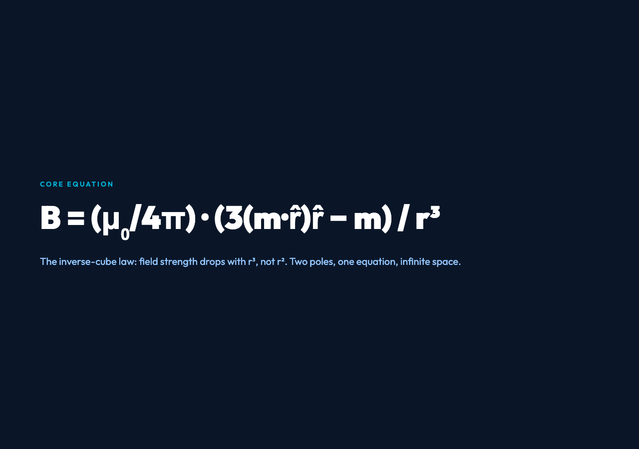
The magnetic field of a dipole at position r from the center, with dipole moment m, is:
B = (μ₀ / 4π) · (3(m·r̂)r̂ − m) / r³
where: – μ₀ is the permeability of free space (4π × 10⁻⁷ H/m) – m is the dipole moment vector (magnitude × direction) – r̂ is the unit vector pointing from the dipole center to the field point – r is the distance from the dipole center
The denominator r³ is the key — field strength drops with the cube of distance, not the square. This is different from gravity or electrostatic monopole fields, which fall off as 1/r². The dipole geometry is special: it produces a field that thins out faster with distance, but with a much richer directional pattern.
The numerator (3(m·r̂)r̂ − m) is what gives the dipole its directional character. When you look along the dipole axis, the field points straight away from (or toward) the dipole. At points perpendicular to the axis, the field points sideways. The field lines form closed loops that enter one pole and exit the other — a topology no crossing rule can break.
What the Visualization Shows
The visualization exposes four layers of the dipole field simultaneously:
Field lines — These are the classic arcing curves that emerge from the north pole and return to the south. The density of lines you see reflects the local field strength: more lines packed together means a stronger field. The simulation draws these by starting small circles near the dipole and integrating the field direction step by step, tracing the path each field line takes. The lineDensity parameter (default: 16) controls how many lines are drawn; increase it and the geometry fills in like contours on a topographic map.
Heatmap — The color-coded field strength map gives you a direct read of |B| at every point. Warm colors mean strong field; cool colors mean weak. The heatmap reveals the characteristic dipole pattern: two bright lobes centered on the poles, with a saddle of weaker field at the equatorial plane perpendicular to the dipole axis. Move the dipole angle and watch the heatmap rotate exactly in sync.
Cross-section planes — The simulation projects the 3D field onto one of three orthogonal planes (xz, xy, or yz). The plane parameter lets you see how the field pattern changes depending on which slice you look at. Along the dipole axis the field is strong and radial; perpendicular to the axis it is weaker and points sideways. Each plane tells a different story about the same 3D structure.
Dipole moment and orientation — The dipoleMoment parameter scales the overall field strength (1.0 is the reference scale). The angleDeg parameter rotates the dipole moment in the x-z plane from 0° (pointing along z) to 90° (pointing along x). Rotating the dipole is the fastest way to build intuition about the directional pattern: every angle gives a completely different field line topology.
Why the Inverse-Cube Law Is the Defining Feature
Most 1/r² fields (gravity, Coulomb’s law for a point charge) create radial field lines that spread uniformly in all directions. The dipole’s 1/r³ law creates a field that thins out faster but with a peculiar consequence: the field at any equatorial point (midway between the poles, perpendicular to the dipole axis) is exactly half the field along the axis at the same distance. That ratio — 1/2 at the equator versus 2/r³ along the axis — is baked into the equation and holds at every distance.

This is why a compass needle aligns with the Earth’s field even though the Earth’s field at the surface is vanishingly small in absolute terms (about 25–65 microtesla). The torque on a magnetic dipole in a field is proportional to the cross product τ = m × B — even a weak field exerts a strong aligning torque if the dipole moment is large enough.
The Geometry No Field Line Can Break
Field lines are a visualization tool, not a physical entity — the field exists continuously in space whether or not you draw lines to represent it. But the no-crossing rule for field lines is a real topological constraint. The reason field lines cannot cross is the same reason streets cannot fork and rejoin: at any point in space the field has a unique direction. Two field lines crossing would imply two different directions at the same point, which is impossible.
This topology is what makes the dipole field so useful as a model. Every magnetic atom is a tiny dipole. A bar magnet is a macroscopic assembly of aligned atomic dipoles, producing a net dipole field. The Sun’s corona ejects plasma along magnetic field lines that map onto interplanetary field geometry. The dipole equation describes all of them — from a refrigerator magnet to a neutron star — with the same three ingredients: moment, direction, distance.
What the Interactive Controls Reveal
The power of the visualization is in what it reveals when you change parameters:
Toggling showFieldLines off/on shows you how much the heatmap alone tells you — and how much the field lines add spatial narrative that the heatmap cannot. Toggling showEquipotential reveals the surfaces of constant magnetic scalar potential, which are orthogonal to the field lines in regions where no current flows. Toggling showVectors overlays arrow glyphs that show the local field direction and magnitude at a grid of points — a more discrete, less artistic version of the same information.
The probe tool (probeX, probeY) lets you hover over any point and read off the exact field components (B_u, B_v) and magnitude at that location. This is where the equation becomes a measurement: you can verify that the field at (r, 90° from axis) is exactly half the field at (r, 0°) at the same distance.
The Field Beneath Every Magnet
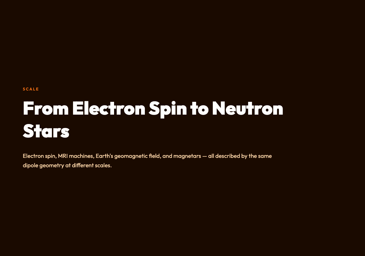
The magnetic dipole field is the simplest model for how magnets work at every scale. At the atomic level, electron spin produces dipole moments. At the human scale, MRI machines use precisely engineered magnetic fields that are variations on the dipole theme. At the planetary scale, the Earth itself is a dipole field generator — with a dipole axis tilted 11° from the rotation axis, which is why a compass needle not only points north but dips downward by an angle that varies with latitude.
The visualization strips all of that down to its essence: rotate the dipole, change the plane, watch the heatmap shift. The equation B = (μ₀/4π) · (3(m·r̂)r̂ − m) / r³ does not get simpler than this — but it never stops being surprising that something so clean can describe something so rich.
The magnetic dipole field is one of the most consequential invisible structures in the universe. From the bar magnet on your desk to the MRI scanner in a hospital to the field protecting Earth from solar wind, the dipole geometry appears at every scale where magnetism matters. What makes it especially elegant is that a single equation — B = (μ₀/4π) · (3(m·r̂)r̂ − m) / r³ — governs all of it: the field strength drops with the cube of distance, the field lines exit the north pole and re-enter the south, and no two field lines ever cross. The visualization makes that equation tangible. Click the dipole, rotate it, watch the heatmap shift. You are looking at the same structure that keeps your compass pointing north.