The Frequency Where Everything Cancels
Tune a radio. You hear one station, not the hundred others your antenna is catching. Somewhere inside the device, a series RLC circuit is doing the work — choosing one frequency from the noise and passing it through. It does this because at one specific frequency, the inductive reactance and the capacitive reactance become equal and cancel. What is left is pure resistance, and the signal passes unimpeded.
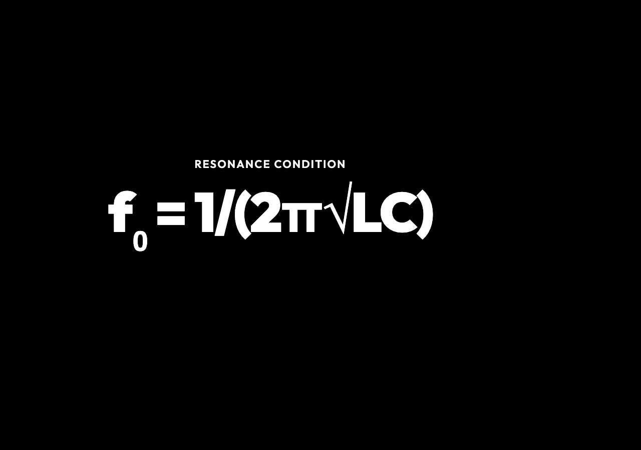
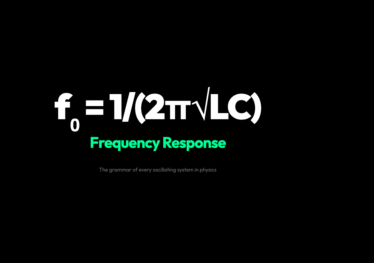
That frequency is called the resonant frequency, written as f₀ = 1/(2π√LC). It depends only on the inductance L and capacitance C — not on the resistance R. The resistance R shapes everything else: how sharp the peak is, how wide the passband, how quickly the phase swings from +90° to −90°.
This is the grammar of every second-order system in physics. The same mathematics describes a mass-spring-damper, a pendulum, an optical cavity. The RLC circuit is the clearest place to see it.
What the Bode Plot Actually Shows
A Bode plot is two graphs that share the same logarithmic frequency axis. The magnitude plot shows 20·log₁₀|H(f)| in decibels. For this series RLC bandpass circuit, 0 dB is the peak — unity gain at resonance where the output voltage across R equals the input amplitude. Negative decibels mean the circuit is attenuating.
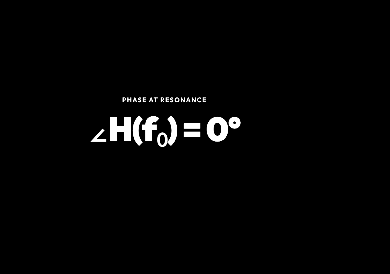
The phase plot shows ∠H(f) in degrees. At low frequency the circuit is capacitive: the capacitor dominates, current leads voltage, and the phase sits near +90°. At resonance it passes through 0° — current and voltage are in phase. At high frequency the inductor dominates, current lags, and phase approaches −90°.
Move the resistance slider and you see something counterintuitive: the resonant frequency f₀ does not move. R controls only the height and width of the peak. Higher R means lower Q, wider bandwidth, a flatter response. Lower R means higher Q, a sharper peak, and more selective frequency filtering.
Move L or C and the resonant frequency shifts. Double C and f₀ drops by a factor of √2. Halve L and f₀ rises by a factor of √2. The shape stays the same form — only the frequency scale changes.
Q Factor: The Measure of Selectivity
Q = (1/R)√(L/C) — the quality factor — is the single number that tells you how sharply a circuit selects its frequency. A radio station at 98.3 MHz with Q = 50 picks a bandwidth of only 1.97 MHz, keeping adjacent stations cleanly separated. An audio crossover handling 20 Hz to 20 kHz needs a low-Q response so one band does not drop off before the next one starts.
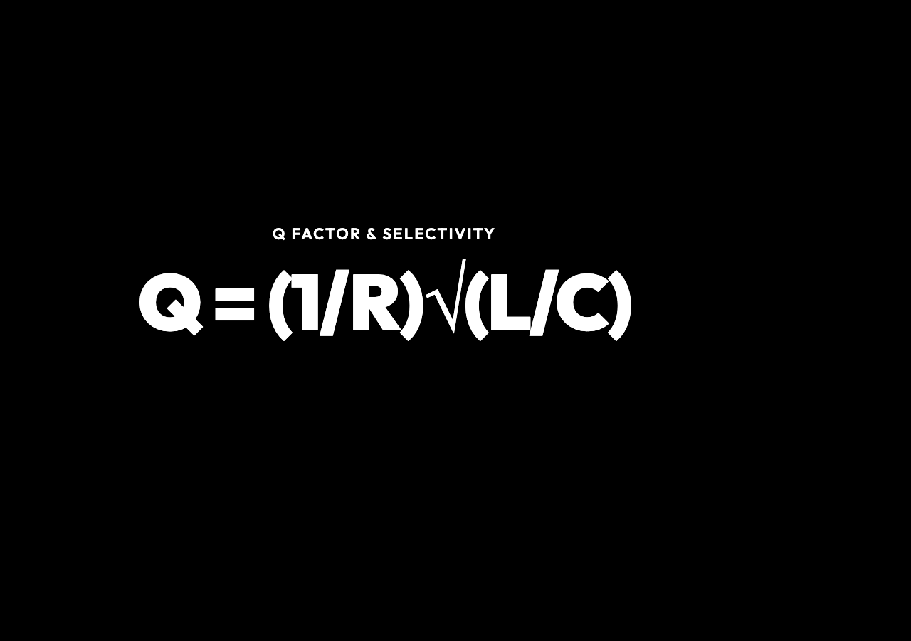
The −3 dB bandwidth is Δf = f₀/Q. This is the frequency range where |H| stays above 1/√2 of its peak — the range where the circuit still “passes” the signal with less than half the power lost. Outside that range, attenuation ramps up at 20 dB/decade — a tenfold frequency change produces a tenfold voltage change.
Where This Physics Appears in the Real World
Radio tuning is the most direct example. An LC tank selects the carrier frequency of the station you want. The Q determines how well the radio rejects the neighboring station on the dial. Higher Q means better selectivity but a narrower capture range — trade-offs that every radio designer manages.
Audio crossover networks in speakers use RLC filters to split the full audio spectrum. A tweeter gets only the high frequencies (a high-pass filter), a woofer gets only the bass (a low-pass filter), and the midrange driver gets a bandpass. The crossover frequency and Q factor set how smoothly these transitions happen — a poorly designed crossover creates peaks and dips that color the sound.
LC oscillators set the clock frequency in computers, microcontrollers, and RF synthesizers. The resonant tank determines the oscillation frequency; the Q determines how stable it is against temperature drift and component variation. A quartz crystal oscillator is a piezoelectric resonance with an extraordinarily high Q — the same second-order physics, but with mechanical rather than electromagnetic storage.
EMI filters use series LC traps to suppress conducted electromagnetic interference at specific frequencies. If a switching power supply generates noise at 150 kHz, a carefully tuned LC trap attenuates it before it leaves the circuit board. The same resonance math, applied to electromagnetic compatibility.
Reading the Plot in Practice
Use the Sharp Resonance preset as a starting point. The magnitude plot shows a tall, narrow peak at f₀. The phase plot shows a steep transition through 0°. The stats panel reads Q, bandwidth, and characteristic impedance Z₀ = √(L/C).
Switch to the Broad Response preset. The peak flattens and widens. Q drops. The phase transition smooths out. What you are seeing is the same circuit with higher resistance — the resonance is still there, but it is less selective.
Try the Audio Filter preset to bring the resonant frequency into the audible range. Notice how the same physics that lets a radio isolate one station from hundreds now shapes the bass response of a speaker system.
Drag the R slider and watch Q and bandwidth change while f₀ stays fixed. Then drag L or C and watch f₀ move while the peak shape follows R. This is the fundamental split: L and C set the frequency scale, R sets the sharpness. That split is the same in every second-order system — whether it is an RLC circuit, a mass on a spring, or a Fabry-Perot optical cavity.
The Grammar Behind the Graph
Every second-order system has the same transfer function structure: a numerator that sets the type of response (bandpass, low-pass, high-pass) and a denominator that carries the resonance. The RLC bandpass has H(jω) = R / (R + jωL + 1/jωC). Set ω = ω₀ = 1/√LC and the imaginary terms cancel — the transfer function simplifies to H = 1. The phase cancels to 0°. This is resonance.
The denominator’s jωL − j/(ωC) term is what creates the resonance. It is the same term that appears in the harmonic oscillator differential equation: the restoring force minus the damping force. The Bode plot is the frequency-domain portrait of that same competition between storage and dissipation.
Understanding how to read it — magnitude in decibels, phase in degrees, Q as the sharpness of the peak, bandwidth as the −3 dB span — is not just useful for circuits. It is the vocabulary for every oscillatory system in physics and engineering.
At resonance, the phase crosses zero — the current and voltage lock in step, and the circuit hums at exactly the frequency the inductors and capacitors agreed on. That single crossing point is where oscillators keep time, radios tune to a voice, and your phone isolates the signal from noise. The Bode plot makes that invisible handshake visible: two curves that tell you everything about what a circuit lets through, and what it swallows whole. Understanding second-order frequency response is not just an exercise in circuit theory — it is the grammar of every system that oscillates, resonates, or filters.