
Combine capacitors, compute reactance, and read the RC time constant off a single result card — without re-deriving the formulas every time. A typical electronics bench moment goes like this: you have three caps in your hand, a 10 kHz square wave on the scope, and the question is what value of capacitance the network actually presents at that frequency. The Elysia Tools Capacitor Calculator takes that whole problem in one shot — paste your capacitor list, pick series or parallel, set the frequency, and read the equivalent capacitance, the capacitive reactance Xc, and the RC time constant together, with the math laid out in the result card instead of buried behind a wall of fractions.
Why a dedicated tool beats re-typing formulas
Three tasks show up over and over in hobbyist and pro electronics work, and each one has its own pothole when done by hand:
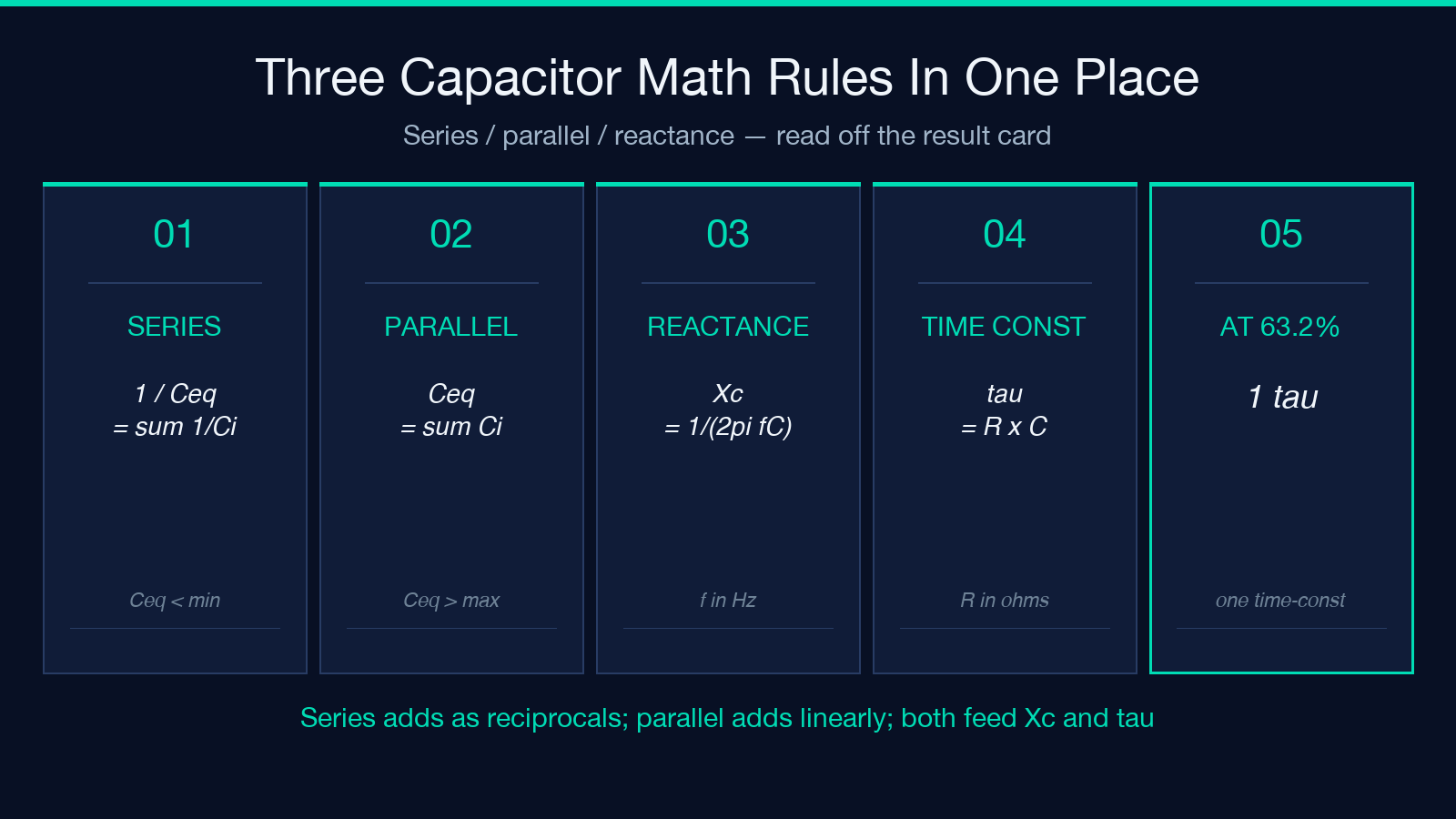
- Combining N capacitors into one equivalent value when the network is series vs parallel — the rules invert between the two modes (1/C = Σ 1/Ci for series, C = Σ Ci for parallel), and a sign-mode slip turns the answer by an order of magnitude.
- Converting a capacitance value at a given frequency into capacitive reactance Xc = 1/(2πfC), which is the AC-circuit analog of resistance.
- Computing the RC time constant τ = R·C, the figure that tells you how fast a capacitor charges to 63.2% of its final voltage through a given resistor.
The first two are the combination rules and the AC-frequency analog of resistance; the third is the time-domain answer that powers every RC filter and integrator on the bench. The tool handles all three on one screen with the same input list, and it draws a network schematic plus a reactance-vs-frequency curve so you can sanity-check the number visually. That is what makes it a field guide instead of a one-off formula lookup. The remainder of this article walks through the math, the practical gotchas, and the worked examples that show the difference between a textbook answer and a bench-ready answer.
Series and parallel: the rule that flips on you
The single most common capacitor mistake is mixing up the two combination rules. The mental shorthand is short and worth memorizing:
- Series capacitors add as reciprocals. 1/C_eq = Σ 1/C_i, which always makes C_eq < min(C_i). The smallest capacitor in a series string dominates the equivalent value, and it also drops the largest share of an applied AC voltage (V_i ∝ 1/C_i).
- Parallel capacitors add as plain numbers. C_eq = Σ C_i, which makes C_eq > max(C_i). All branches see the same voltage, so current divides inversely with capacitance.
The reason the series/parallel Capacitor Calculator is structured as a mode toggle is precisely to force you to pick one rule before computing. The result card then prints the equivalent capacitance together with the network schematic (series or parallel), so the visual matches the math you just applied. A worked example: four 10 µF caps in parallel give 40 µF (the rule is linear), while the same four in series give 1 / (4 · 1/10µF) = 2.5 µF (the rule is harmonic-mean shaped). The difference is exactly a factor of 16, and switching the mode toggle is the single most reliable way to avoid losing that factor.
Reading capacitive reactance Xc at any frequency
Capacitive reactance is the AC analog of resistance and tells you how strongly a capacitor opposes sinusoidal current at a given frequency. The relationship is Xc = 1 / (2π · f · C), which has two important shapes:
- At a fixed capacitance, Xc falls as frequency rises — a 1 µF cap is about 159 Ω at 1 kHz but only 1.59 Ω at 100 kHz. That is why bypass caps on digital rails work: at high frequency they look like a short to ground.
- At a fixed frequency, Xc falls as capacitance rises — doubling C halves Xc. Designers use this when picking a coupling cap: larger C extends the low-frequency response.
The tool’s reactance mode takes a single capacitance and a frequency, computes Xc in ohms, and overlays a log-log Xc-vs-frequency curve with the chosen frequency marked. The curve is what makes a “feels right” answer into a measured one — you can slide frequency up by a decade and watch Xc drop by the same decade, then read the actual numeric at any point. For a quick sanity check, a 100 nF cap at 1 kHz should sit close to 1.59 kΩ; if the curve shows something else, the value or the frequency is wrong before any component is soldered in.
The RC time constant τ = R·C
The third leg of the tool is the RC time constant, the figure that governs how fast a capacitor charges through a resistor toward its final voltage. The relationship is τ = R · C, with the corollary that a capacitor reaches 63.2% of its final voltage after one τ, 86.5% after 2τ, 95.0% after 3τ, and 98.2% after 4τ — the same exponential charging curve that powers every RC low-pass filter, integrator, and timer in analog electronics.
Enter a series resistor value in the tool’s optional field and the result card prints τ in seconds, with the assumption that you are charging C_eq (or the single capacitor, in reactance mode) through that resistor. A worked example: a 10 kΩ resistor feeding a 100 µF cap gives τ = 1 second, which means a 5 V step hits 3.16 V after one second and 4.75 V after three seconds. The same RC product is also the cutoff period for an RC low-pass filter (f_c = 1 / (2π · R · C)), so the time-constant number doubles as a frequency-domain answer. The tool does not print f_c directly, but the formula is one line away once τ is on screen.
Worked example: a 3-cap decoupling network
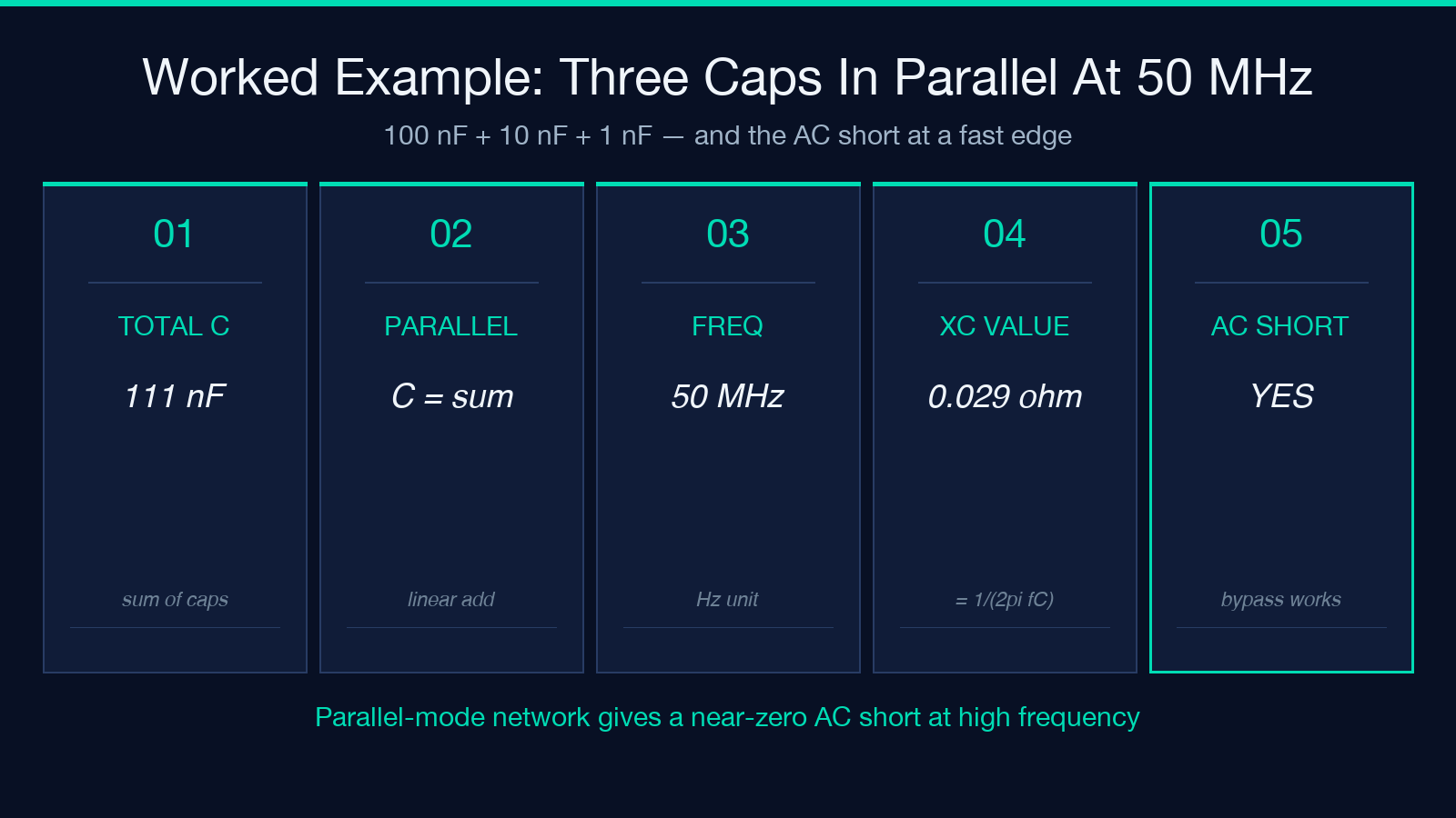
Picture a small mixed-signal board with a 100 nF, a 10 nF, and a 1 nF cap all on the same supply rail, in parallel. The parallel-mode answer is the trivial one: 100 + 10 + 1 = 111 nF. The interesting question is what happens at the frequency of a fast edge — say 50 MHz. Plug the 111 nF total into reactance mode at 50 MHz, and Xc = 1 / (2π · 50e6 · 111e-12) ≈ 0.0287 Ω. That is the “AC short” behavior the decoupling network is supposed to provide, and the number reads straight off the result card.
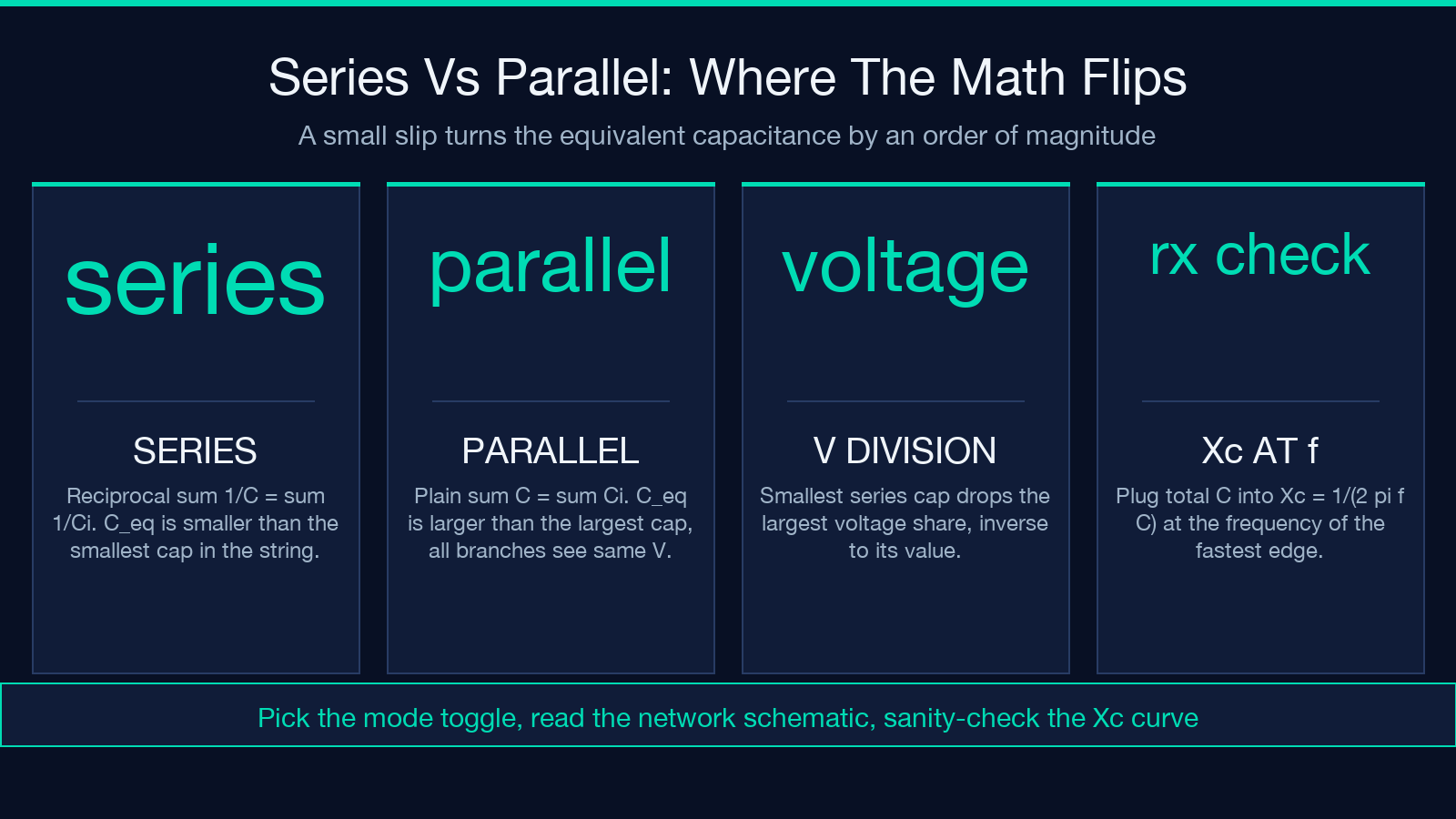
Now reverse the perspective. Take the same three caps and imagine them inadvertently in series (a wrong footprint, a bridged trace). The series-mode answer is 1 / (1/100nF + 1/10nF + 1/1nF) = 1 / (1.11e10) ≈ 0.9 nF. The AC short at 50 MHz drops to about 3.5 Ω — still low, but a hundred times worse than the parallel case, and high enough to be visible as ringing on a fast edge. This is the scenario the mode toggle exists to prevent.
Edge cases and unit pitfalls
Three small traps catch people the first time they combine capacitors:
- Unit prefixes. Capacitor values are routinely written with prefixes that span twelve orders of magnitude — 1 pF (10^-12 F) to 1 F (supercap range). The tool accepts standard SI prefixes (
p,n,uorµ,m,k) and treats uppercase/lowercase the same. A common slip is reading “100” as 100 F when the BOM meant 100 nF — always check the prefix before committing the network to the schematic. - Series voltage division. In a series string, the smallest capacitor drops the largest share of the voltage. If you put 1 µF and 10 µF in series across a 10 V source, the 1 µF drops about 9.1 V and the 10 µF drops about 0.9 V — reverse of intuition if you have only ever worked with resistors. The tool’s voltage-shares output (when applicable) is the place to read that off directly.
- Frequency units. Reactance assumes the frequency is in Hz, not kHz or MHz. A common typo is entering 10 when the intended value is 10 kHz — the resulting Xc is 1000x too small, and the reactance-vs-frequency curve is shifted left by three decades. The tool’s frequency field is explicitly labeled in Hz, but double-checking before reading the Xc off the curve saves a re-run.
How to read the result card
The tool returns all three numbers (C_eq, Xc, τ) on a single result card, plus a network schematic and a reactance-vs-frequency curve where applicable. Three patterns help you read it quickly:
- The C_eq line shows the equivalent capacitance in SI-prefixed farads (pF / nF / µF / mF / F), so 111 nF reads as “111 nF” rather than “0.000000111 F”. The unit picker matches the prefix you typed in the input list, so the rounded answer reads naturally.
- The Xc value appears only when you supplied a frequency, and it sits on the same row as C_eq so you can confirm the relation (Xc = 1/(2πfC)) at a glance. If the Xc number looks wrong by a factor of 1000, double-check the frequency unit (Hz vs kHz vs MHz).
- The τ value appears only when you supplied a series resistor. It is shown in seconds (or the appropriate SI prefix for very long / very short time constants), and is rounded to three significant figures to avoid implying false precision.
What pairs naturally with a capacitor calculator
Capacitor networks rarely live alone on a schematic. Two adjacent tools round out the workflow:
- For a passive low-pass filter built from the same RC pair, the RC time constant doubles as the cutoff-period input, and f_c = 1/(2πτ) is one division away.
- For inductor networks on the same board (LC filters, switching converters), the same series/parallel reactance math applies but with X_L = 2πfL instead of Xc — the structural pattern transfers even though the formula inverts.
The full set of math and numbers tools at Elysia Tools includes both this calculator and a wider bench of electrical-engineering utilities, all built on the same input-and-result-card pattern. For more field guides and worked examples, browse the Elysia Tools library.
