
The classic 9:3:3:1 dihybrid ratio is the opening move, not the endgame. Once a second gene masks, suppresses, or duplicates the first, the F2 phenotypic ratio reshapes into one of seven canonical patterns — 9:7, 9:3:4, 12:3:1, 13:3, 15:1, 9:6:1, or stays at 9:3:3:1 — and every downstream chi-square, every linkage test, every breeding-program decision rides on getting that ratio right before you count a single offspring. A misread 9:3:3:1 where the data actually shows 9:7 collapses the chi-square goodness-of-fit into nonsense, and the rest of the lab notebook follows.
The Epistasis Ratio Calculator treats all seven gene-interaction patterns as named selectors, so the biologist names the interaction (recessive epistasis, dominant suppression, complementary genes), enters observed counts, and the tool returns expected counts, per-class probabilities, and the chi-square statistic against the critical values 3.841 / 5.991 / 7.815 at α = 0.05. The seven ratios reduce to one workflow once you know what to look for — and that is the field guide this article gives you.
What epistasis means and the seven canonical F2 ratios
Epistasis is gene interaction where the allele at one locus masks or modifies the expression of alleles at another locus. The F2 generation still segregates 9:3:3:1 at the genotype level (two independent loci, each heterozygous Aa Bb, give 16 equally-likely genotype combinations), but the visible phenotype collapses into fewer classes because one gene’s output overrides the other’s.
The mechanism matters more than the memorization. In complementary genes (9:7), both loci contribute a step in the same biosynthetic pathway — knock out either gene, the pigment does not form, the flower stays white. In recessive epistasis (9:3:4), the homozygous recessive at one locus produces a yellow seed coat regardless of the other gene’s alleles — the 9 green-round, 3 green-wrinkled, 3 yellow-round, 1 yellow-wrinkled from the textbook 9:3:3:1 collapses to 9 green:3 green-wrinkled:4 yellow because the yellow-wrinkled class (1) and the yellow-round class (3) merge into “yellow”. The numerical collapse is the diagnostic — if your F2 reads as three classes with the dominant phenotype in the largest class and a 9:3:4 split in the residual, you have recessive epistasis.
Seven canonical patterns cover the field. The dihybrid baseline 9:3:3:1 is the no-interaction case. 9:7 complementary genes (both loci required for one product). 9:3:4 recessive epistasis (homozygous recessive at locus B masks A). 12:3:1 dominant epistasis (a dominant allele at locus A masks B). 13:3 dominant suppression (a dominant allele at one locus suppresses the other). 15:1 duplicate dominants (either dominant allele produces the same phenotype). 9:6:1 cumulative duplicates (both dominants together intensify the trait, each dominant alone produces a weaker form).
The right way to pick a pattern: count the visible F2 classes first. Two classes means 15:1 or 13:3 (suppression). Three classes means 9:7, 9:3:4, 12:3:1, or 9:6:1. Four classes means 9:3:3:1. The size of the dominant class relative to the rest disambiguates within the three-class group — 9 of 16 is recessive epistasis or complementary, 12 of 16 is dominant epistasis, and 9:6:1 has a 9:6 split rather than 9:7 or 9:4. The calculator encodes this logic as named presets, so you stop counting classes manually and let the tool project the expected distribution from the named interaction.
Counting offspring and what to feed the calculator
The calculator’s input is observed counts per phenotype class, not a probability or a ratio string. For a 9:3:4 recessive-epistasis cross with 240 F2 offspring, the expected distribution is 135 : 45 : 60, and you enter whatever you actually counted in the three classes. The tool does the multiplication and reports the expected count, the per-class probability, and the chi-square statistic with degrees of freedom = (number of classes − 1).
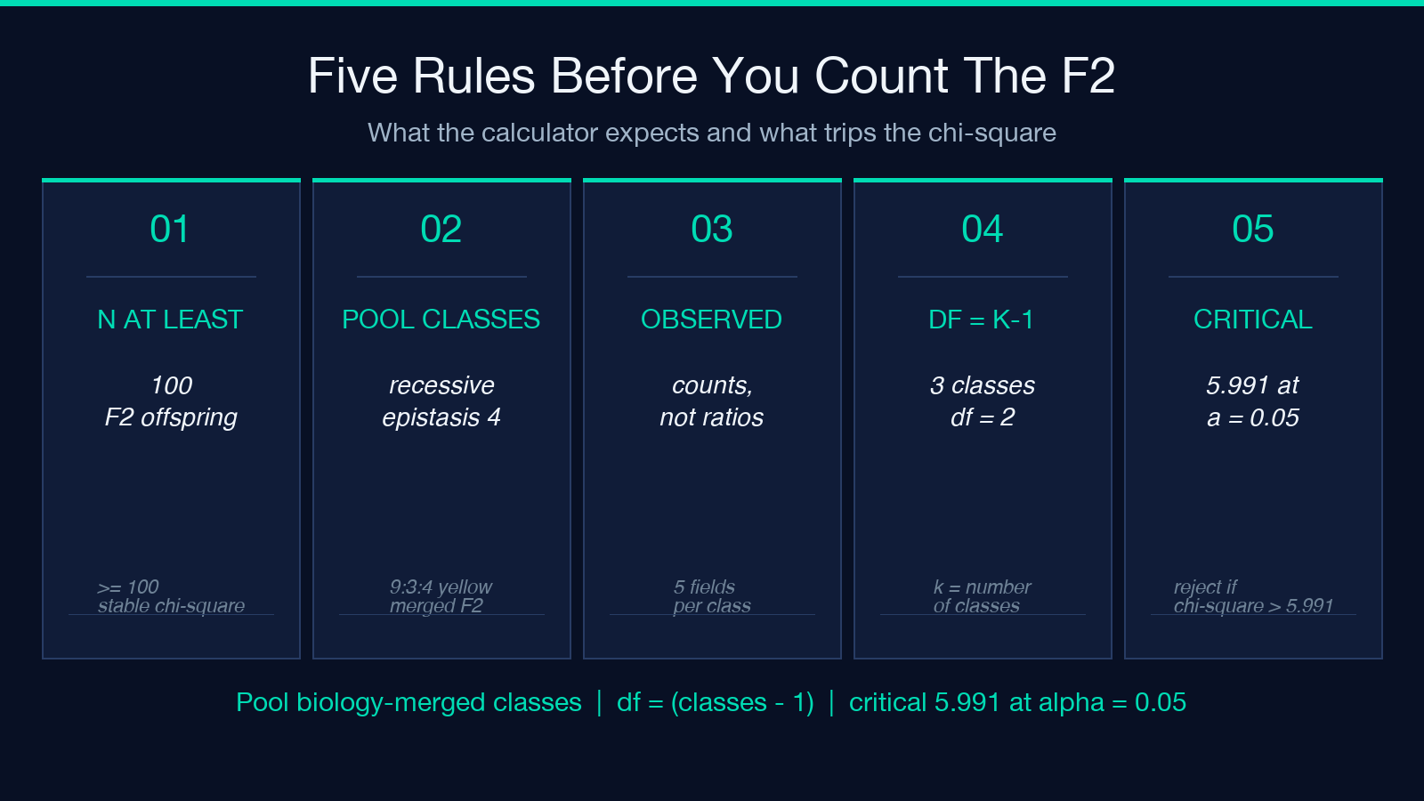
Two practical rules before you count. First, count to at least 100 offspring before trusting the ratio — small samples make any chi-square unstable and the 3.841 critical value at df=1 will reject legitimate 9:3:3:1 crosses by chance alone. Second, pool classes that the biology merges — if the interaction is recessive epistasis, the yellow-round and yellow-wrinkled F2 individuals are one phenotype from the standpoint of the ratio test, even though the genotype underneath differs. Forgetting to pool inflates df and deflates chi-square.
The calculator exposes both the per-class expected count and the total. A 9:3:4 with 240 F2 gives 135 expected green, 45 expected green-wrinkled, 60 expected yellow. If your observed is 140:38:62, the chi-square is small and you fail to reject 9:3:4. If your observed is 110:38:92, the chi-square is large and you reject — and the next step is to ask whether 9:3:4 was the right interaction in the first place.
The chi-square goodness-of-fit in five steps
The chi-square test asks a single question: does the observed distribution match the expected distribution under the named ratio, or does the deviation exceed what chance alone would produce? Five ordered steps give you the answer without skipping any bookkeeping.
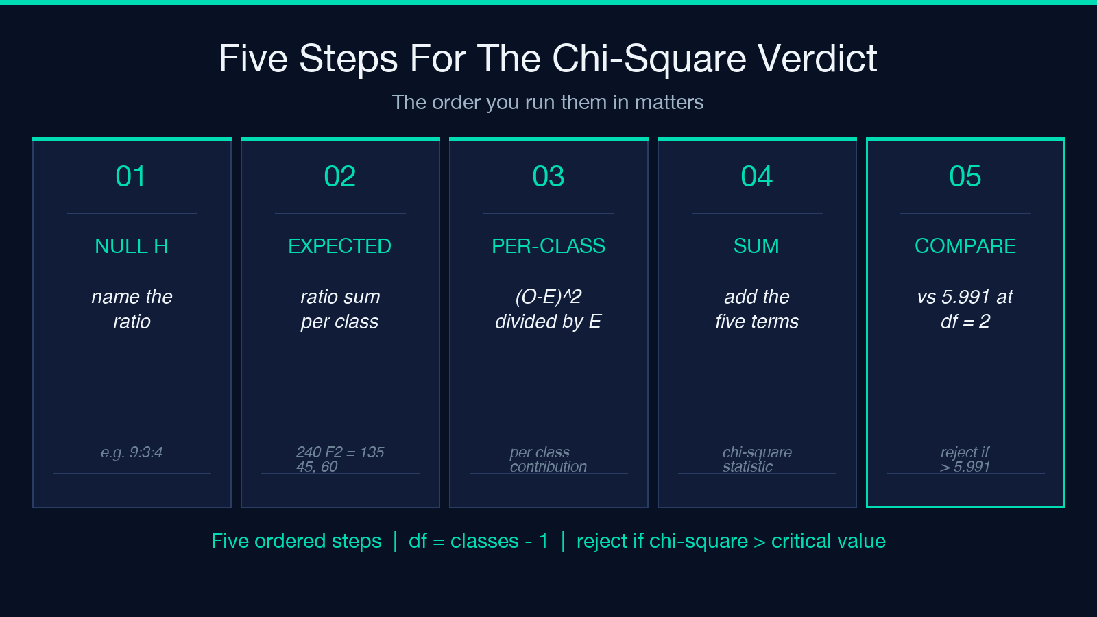
Step 1 — write the null hypothesis. “The F2 follows the named ratio (e.g., 9:3:4).” Step 2 — compute expected counts as (ratio sum / total offspring) × per-class ratio, so a 9:3:4 with 240 F2 gives expected = (16/16) × 240 × 9/16, 3/16, 4/16 = 135, 45, 60. Step 3 — for each class compute (observed − expected)² / expected. Step 4 — sum the per-class contributions to get chi-square. Step 5 — compare against the critical value at df = (classes − 1) and α = 0.05: 3.841 for df=1 (two-class ratios), 5.991 for df=2 (three-class ratios), 7.815 for df=3 (four-class ratios). If chi-square exceeds the critical value, reject the null — the F2 does not fit the named interaction.
The calculator reports chi-square and the critical value side by side so you can verify the rejection decision without flipping to a stats table. The 5.991 cutoff for three-class ratios is the one most F2 crosses land on.
When the chi-square rejects — and what to do next
A rejected null is not a failed experiment; it is information. The named interaction was wrong, or the F2 sample is contaminated by a second ratio you did not account for, or the inheritance is more complex than two loci with one interaction.
Three diagnostic branches. First, try a different named interaction. If 9:3:4 was rejected, test 9:7 (complementary genes) or 12:3:1 (dominant epistasis) on the same data — only one of the three-class ratios will fit, and the fit tells you the biology. Second, check for linkage. Two genes on the same chromosome do not segregate independently, the 9:3:3:1 baseline fails, and the F2 ratio skews toward the parental phenotypes. The calculator’s named interactions all assume independent assortment, so a persistent rejection across all seven named ratios is a linkage signal. Third, count again. Off-by-one errors in phenotyping collapse the chi-square in unpredictable ways; a recount by a second observer usually resolves borderline cases.
The calculator lets you re-run the same observed counts against any of the seven named interactions without retyping the numbers, so the diagnostic cycling is cheap. A clean 9:3:4 fit and a clean 12:3:1 fit on the same data is impossible — only one interaction produces the observed three-class split. Pick the one that fits, report the named interaction, and the F2 ratio is settled.
Worked example: a 9:3:4 cross with 240 F2 offspring
Suppose you cross two heterozygous F1 plants (Aa Bb × Aa Bb) where locus B is recessive epistatic to locus A — homozygous bb produces yellow seeds regardless of the A locus alleles. You count 240 F2 seeds: 142 green-round, 38 green-wrinkled, 60 yellow. The expected ratio is 9:3:4, giving expected counts 135 green-round, 45 green-wrinkled, 60 yellow.
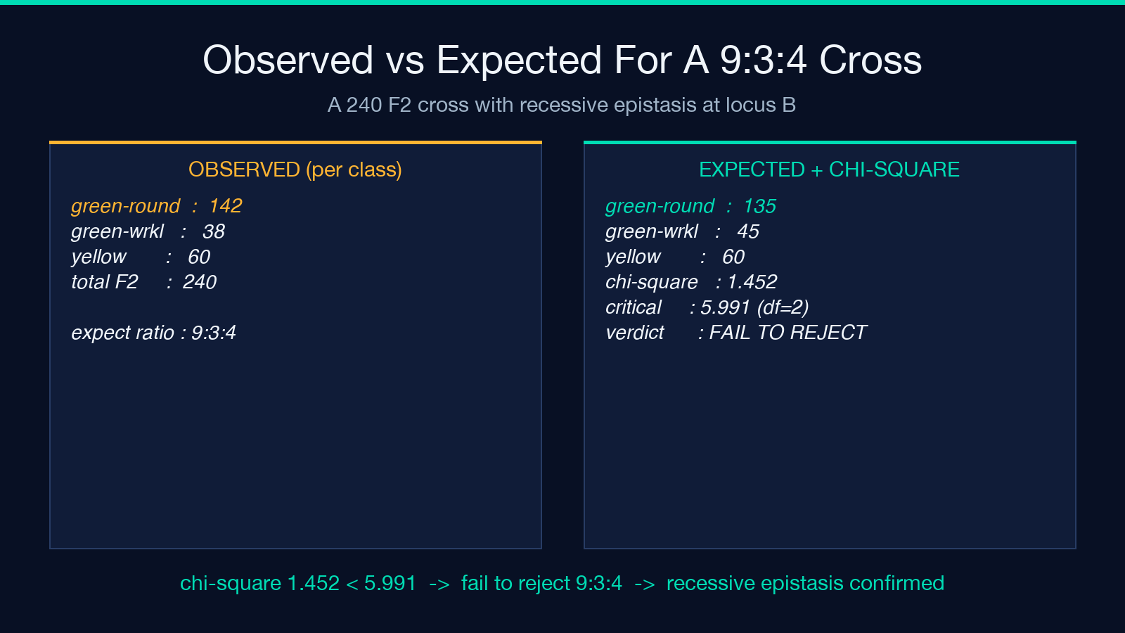
Compute chi-square: (142−135)²/135 = 49/135 = 0.363; (38−45)²/45 = 49/45 = 1.089; (60−60)²/60 = 0. Sum = 1.452. Degrees of freedom = 2 (three classes minus one), critical value at α=0.05 is 5.991. Observed 1.452 is well below 5.991 — you fail to reject the 9:3:4 hypothesis, and the cross behaves as recessive epistasis. The 38 vs 45 expected in the green-wrinkled class is within sampling noise for n=240.
If instead the observed was 110:55:75, chi-square becomes (110−135)²/135 = 625/135 = 4.63; (55−45)²/45 = 100/45 = 2.22; (75−60)²/60 = 225/60 = 3.75. Sum = 10.60. Reject 9:3:4 (10.60 > 5.991). Try 9:7 on the same data: expected 135:105, chi-square = (110−135)²/135 + (130−105)²/105 = 4.63 + 5.95 = 10.58. Also reject. The F2 is not a clean two-locus epistasis cross — time to check for a third locus, a linkage distortion, or a phenotyping boundary you drew wrong.
The calculator’s input form lets you re-key observed counts against any of the seven named interactions in seconds, so the diagnostic cycling from 9:3:4 to 9:7 to 12:3:1 is one form-resubmit per hypothesis. The output always reports expected counts, chi-square, critical value, and the reject / fail-to-reject verdict together.
Pairing the ratio test with a sample walk-through
The cleanest way to internalize the seven canonical F2 ratios is to see one worked example for each, not just the 9:3:3:1 baseline. The Epistasis Ratio Calculator lets you pick a named interaction from a dropdown, type observed counts, and read the chi-square verdict — so the workflow is the same whether the ratio is 9:7 (sweet pea flower color), 13:3 (chicken feather color), or 15:1 (grain color in some wheat crosses).
For a 9:7 sweet-pea cross with 200 F2, the expected split is 112.5 white-flower (no functional enzyme at either locus) and 87.5 purple-flower (functional at both). If your observed is 120:80, chi-square is small and you fail to reject — both loci carry complementary steps of the pigment pathway. For a 13:3 chicken cross with 160 F2, expected is 130 colored:30 white-suppressed; an observed 125:35 fails to reject 13:3. The shape of the rejection across all seven ratios is the diagnostic, and the calculator makes the rejection cheap to test.
The pairing that matters: the named interaction identifies the biology, the chi-square confirms whether your observed data is consistent with that biology, and a rejected null forces you to re-examine both the interaction type and the phenotyping boundary. The calculator’s seven-ratio preset covers the field; if your F2 fails all seven, the inheritance is two-locus-plus-linkage, polygenic, or cytoplasmic — none of which a single two-locus model can settle.
Common failure modes when reading an F2 ratio
Three mistakes show up over and over in epistatic-cross interpretation. First, treating 9:3:3:1 as the default. It is the no-interaction baseline, not the universal expectation. Any cross where two genes interact — and most do — produces a different ratio, and assuming 9:3:3:1 on data that is actually 9:7 or 13:3 inflates chi-square to a guaranteed rejection. Second, using the wrong degrees of freedom. A 9:3:4 cross has three visible classes, so df=2, critical value 5.991 — not df=3 and not 7.815. Off-by-one in df flips borderline verdicts the wrong way. Third, forgetting to pool classes that biology merges. Recessive epistasis gives yellow-round and yellow-wrinkled as one yellow phenotype from the ratio standpoint, even though two genotypes underlie it; pooling reduces df from 3 to 2 and is the difference between a clean 9:3:4 fit and a guaranteed rejection.
A secondary failure mode is sample size. With 50 F2, the expected 9:3:4 split is 28.1:9.4:12.5 — the 9.4 expected in the second class is small enough that an observed count of 5 vs 14 will fail any chi-square regardless of whether 9:3:4 is correct. Sample up before testing.
The calculator lets you enter any n and any ratio; the per-class expected count and the chi-square update live. For borderline n=50 crosses, the tool’s chi-square verdict is a flag that the sample is too small, not a verdict on the biology. Re-test at n=200 before committing to a rejected null.
Closing note: the seven ratios, one workflow
Epistasis looks like seven different problems because the F2 phenotypic splits differ. Mechanically it is one problem — name the interaction, count the F2, run the chi-square — and the Epistasis Ratio Calculator reduces the seven problems to seven dropdown options on one form. The decision tree is class-count first (two, three, or four visible phenotypes), dominant-class size second (9, 12, 13, or 15 of 16), and named interaction third. The chi-square goodness-of-fit confirms the named interaction against the observed data, and a rejected null is the start of the next diagnostic cycle, not the end of the experiment.
The calculator cites the underlying population genetics — Mendel 1866, Bateson & Punnett 1905, Griffiths/Hartl/Clark 2007 — so the named interactions are not heuristic guesses but the textbook canonical patterns. Educational use only, as the tool’s footer notes: the calculator is for genetics coursework, problem-set verification, and lab-notebook cross-checks, not for clinical or breeding-program decisions where the F2 sample is small and the biology may include linkage, epistasis-plus-modifier, or three-locus interactions outside the seven-ratio model.
For a full reference of the seven ratios, observed-vs-expected chi-square workflows, and an interactive form that handles any F2 sample size, see the calculator page. For more education and genetics tools, browse the Elysia Tools catalog.
