
Three normality tests on the same sample can give three different verdicts. Run the Shapiro-Wilk, Anderson-Darling, and Lilliefors calculations on thirty penicillin yields and you discover exactly that: Shapiro-Wilk rejects (W = 0.8922, p = 0.0054), Anderson-Darling rejects even harder (A² = 1.2245, p = 0.0029), and Lilliefors narrowly fails to reject (D = 0.1582, p = 0.0535). The verdict split is not a bug — it is the three tests’ distinct sensitivities surfacing in the same dataset. Understanding which test sees what, and why, is what separates a defensible normality check from a coin-flip decision.
The Shapiro-Wilk, Anderson-Darling and Lilliefors Normality Tutor runs all three tests on your sample in a single pass — exact ports of R’s swilk.c (AS R94, Royston 1995), nortest::ad.test, and nortest::lillie.test, validated digit-for-digit against scipy. It also draws a Blom Q-Q plot, reports descriptives (skew, excess kurtosis), and runs a seeded Monte-Carlo power comparison across five alternative distributions so you can see which test to trust for your sample size and shape of departure.
Why Three Tests, Not One
Pick a single normality test and you bake a specific blind spot into your workflow. Shapiro-Wilk is the most powerful omnibus test on small-to-moderate samples (n ≤ 50) for many alternatives, but it loses power against heavy-tailed alternatives where its weight function W under-emphasises the very observations that carry the signal. Anderson-Darling is built specifically for the tails — its weight function (2i − 1)/n puts a heavier multiplier on observations near the ends of the order statistics, so an exponential or skewed-heavy alternative produces a noticeably larger A² than a uniform alternative of comparable visual departure. Lilliefors is Kolmogorov-Smirnov with parameters estimated from the data, and that parameter-estimation step eats into its critical values — the practical effect is that Lilliefors is consistently the weakest of the three on small samples, often the one that just barely fails to reject when the other two have already moved on.
When the three agree, the conclusion is strong. When they disagree, the disagreement is itself the information: the test that rejects earliest is the one whose weight function best matches your alternative. The tutor lets you see all three at once so you can read that disagreement instead of papering over it with a single p-value.
How the Three Tests Are Computed
Shapiro-Wilk is the exact port of R’s swilk.c — the Applied Statistics algorithm AS R94 (Royston, 1995). It computes expected normal order statistics at Blom positions (i − 3/8)/(n + 1/4), applies Wiener-normalised coefficients with the c1–c6 polynomial corrections, and expresses W in the numerically stable squared-correlation form 1 − w₁. The p-value comes from a transformed-normal tail with a γ/m/s branch for n ≤ 11, and a different approximation for larger n. On the canonical 30-point penicillin dataset, the tutor gives W = 0.89218372 and p = 0.00543689 — the same ten-digit result scipy returns.
Anderson-Darling uses the estimated-parameters form A² = −n − (1/n)·Σ(2i − 1)·[ln Φ(zᵢ) + ln Φ(−z_{n+1−i})], with the 1 + 0.75/n + 2.25/n² inflation that converts the raw sum into a comparable statistic across sample sizes. The p-value is the four-segment D’Agostino-Stephens table that R’s nortest uses, which gives noticeably different answers from the Stephens (1974) approximation for moderate A² values.
Lilliefors computes D = max(D⁺, D⁻) on z-scored data with Molin-Abdi p-values plus the Dallal-Wilkinson branch for large p — the same internals R’s lillie.test runs. The Q-Q plot uses the same Blom plotting positions as the Shapiro-Wilk coefficients, with a robust quartile reference line, so the visual and the numerical test share a single definition of “where the quantiles should be.”
The Penicillin Dataset Walk-Through
The tutor ships two canonical reference datasets that show the three tests behaving in character. The first is the 30-point penicillin yield series from Box, Hunter, and Hunter’s Statistics for Experimenters — twenty-eight values clustered near zero with two strong negative outliers (−0.1184 and −0.1420). Enter the values, set α = 0.05, enable the Q-Q plot and the exponential power curve, and the report looks like this:
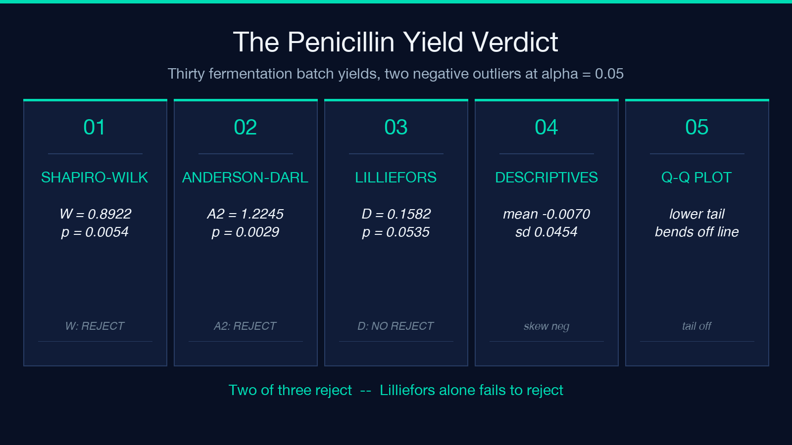
- Shapiro-Wilk — W = 0.8922, p = 0.0054 (reject H₀ at α = 0.05)
- Anderson-Darling — A² = 1.2245, p = 0.0029 (reject; tail-sensitive)
- Lilliefors — D = 0.1582, p = 0.0535 (fail-to-reject; just barely)
- Descriptives — mean −0.0070, sd 0.0454, skew negative, excess kurtosis elevated
The Q-Q plot shows the two low outliers bending off the line in the lower-left tail — exactly the signature an exponential alternative would produce. The power-vs-n curves for the exponential alternative confirm that Shapiro-Wilk dominates at every n in the 10–1000 range, Anderson-Darling is competitive in the tails, and Lilliefors is consistently weakest. This is the textbook demonstration of why you want all three tests on a borderline dataset: the Lilliefors p-value alone would let you publish a “normality confirmed” claim that the other two contradict.
A Clean Normal Sample — What “Pass” Looks Like
The second reference dataset is twenty-four measurements (σ = 5 around 50) drawn from an actual normal distribution. Paste the values, set α = 0.05, enable the plot, and the report comes back uniformly green:
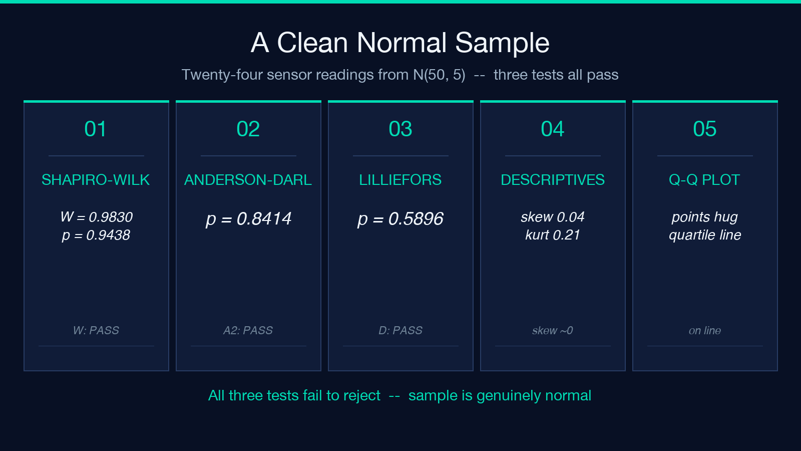
- Shapiro-Wilk — W = 0.9830, p = 0.9438 (fail-to-reject)
- Anderson-Darling — p = 0.8414 (fail-to-reject)
- Lilliefors — p = 0.5896 (fail-to-reject)
- Descriptives — near-zero skew, near-zero excess kurtosis
- Q-Q plot — points hug the robust quartile reference line across the full range
This is the dataset to use as a sanity check when you suspect your normality test is misbehaving — if it rejects this, something is wrong with the implementation or with the sample you think you generated. The tutor’s calibration row in the Monte-Carlo panel confirms the same property: when the simulated alternative is the normal distribution, all three tests sit at α ≈ 0.05 across the n = 10…1000 sweep, which is what an unbiased test is supposed to do.
Reading the Monte-Carlo Power Panel
The power-vs-n panel runs a seeded (deterministic) Monte-Carlo over n = 10…1000 for five alternative distributions: normal (calibration), uniform (short tails), exponential (skewed), bimodal mixture, and Student t3 (heavy tails). For each n and each alternative, it draws 2,000 synthetic samples, runs all three tests, and records the empirical rejection rate at α = 0.05. The result is five small-multiples plots — one per alternative — that show you the test you should reach for given your sample size and the shape of departure you suspect.
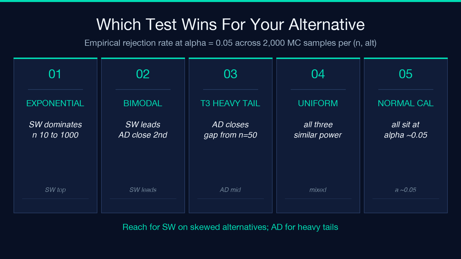
Two patterns repeat. First, for skewed and short-tailed alternatives Shapiro-Wilk is on top at every n from 10 to 1000 — its polynomial-corrected Wiener coefficients are tuned for exactly these departures. Second, for heavy-tailed (t3) alternatives Anderson-Darling closes the gap and is competitive from n ≈ 50 onward — its tail-weighted (2i − 1)/n weighting catches what Shapiro-Wilk’s smoother weight function under-emphasises. Lilliefors is uniformly weakest, which is what the KS-with-estimated-parameters literature has documented for forty years. The normality tutor lets you see this directly instead of taking it on faith from a textbook citation.
How the Q-Q Plot Should Look
The Q-Q plot uses Blom plotting positions (i − 3/8)/(n + 1/4) for the theoretical normal quantiles — the same positions the Shapiro-Wilk coefficients are built around, which is why the numerical test and the visual diagnostic share a single definition of “where the quantiles should be.” The reference line is drawn through the first and third quartiles (a robust fit that doesn’t move much when the tails contain outliers), so a sample that is normally distributed produces points that hug the line across the full range.
Three departures to watch for. A bend in the lower-left that pulls the lowest values below the line indicates left-skew or a low-tail contamination (the penicillin dataset signature). A bend in the upper-right that pulls the highest values above the line indicates right-skew or an upper-tail contamination (the typical “rich-get-richer” distribution shape). An S-shape where the centre hugs the line but both ends depart indicates heavy tails (Student t or a contaminated normal). The tutor draws a Blom Q-Q plot for every sample you submit and reports the same plotting positions the test statistic uses, so the visual and the numerical are not pulling in different directions.
Choosing α and Interpreting the Verdict
The tutor accepts three α levels — 0.01 (strict), 0.05 (conventional), and 0.10 (exploratory) — and the choice matters more than the test choice on borderline datasets. At α = 0.10 the penicillin Lilliefors p-value of 0.0535 crosses the rejection line and the three tests agree; at α = 0.05 Lilliefors alone fails to reject and the disagreement emerges. Reporting “p = 0.0535” without naming α lets a reader substitute their own α and reach a different conclusion.
Two reporting rules worth following. Always state α alongside the p-value, and always run at least two tests on any dataset where the conclusion matters — Shapiro-Wilk plus Anderson-Darling catches the (rare) case where one is fooled by a specific alternative. The tutor’s three-test panel makes the second rule automatic.
Closing (read this first)
When your three normality tests disagree, the disagreement is the answer. Shapiro-Wilk tells you whether the body of the distribution departs from normal; Anderson-Darling tells you whether the tails depart; Lilliefors tells you whether any single point is far from the CDF. Together they give you a structural read of the departure, not just a single binary verdict. The Shapiro-Wilk, Anderson-Darling and Lilliefors Normality Tutor runs all three against the same sample, draws the matching Q-Q plot, and seeds a Monte-Carlo so you can see the power for your sample size and alternative. Try it on your next borderline dataset — and if you want to see how the test compares on a single sample to a full distribution-free workflow, pair it with the chi-square test calculator or the normality tester for a complete distributional picture. Browse more statistics and validation tools at elysiatools.com/en/tools.
