
Two heat exchangers with the same area, same flow rates, and same U-value can move dramatically different amounts of heat depending on how the fluids are routed. The effectiveness-NTU method packs that single fact into one ratio per arrangement, and the Heat Exchanger ε-NTU Calculator implements the four closed-form expressions that thermal designers reach for first: parallel flow, counter flow, shell-and-tube one-two pass, and crossflow both-unmixed. This field guide walks through the five outputs the calculator returns, the three capacity-ratio regimes that change everything, the four arrangement formulas in plain math, the two phase-change edge cases, and the four failure modes the form will silently accept. By the end you should be able to read any ε-NTU problem and predict which lever — C*, NTU, or arrangement — the calculator will turn first.
Why the Effectiveness-NTU Method Replaces the LMTD
The older approach to heat-exchanger rating is the log-mean temperature difference: q = U · A · ΔT_LM, where ΔT_LM is the log-mean of the two end-point temperature differences, corrected by an F factor for non-counter arrangements. That approach works, but it requires knowing the outlet temperatures up front — which is exactly the unknown you are trying to find. The effectiveness-NTU method flips the problem: you supply the geometry (A), the heat-transfer coefficient (U), and the two stream capacity rates (C_h, C_c), and you receive a dimensionless effectiveness ε that tells you what fraction of the thermodynamic maximum is being moved. The actual heat rate is then q = ε · C_min · (T_h,in − T_c,in), and the outlet temperatures fall out by a simple energy balance on each side.
That inversion is the engineering payoff. The LMTD formula needs an iterative solve because ΔT_LM depends on the unknowns you are solving for. The ε-NTU formulas are closed-form: one exponent, one square root, or one polynomial per arrangement, with no iteration required. For a sizing study that compares dozens of arrangements or sweeps U across an order of magnitude, the closed-form path wins on both speed and clarity. The calculator’s job is to evaluate the four closed forms and report whichever one the chosen arrangement asks for.
The Five Numbers You Always Have to Pass In
The calculator exposes five operating inputs and two optional ones. The required five are the hot-side capacity rate C_h (in W/K), the cold-side capacity rate C_c (in W/K), the overall heat-transfer coefficient U (in W/(m²·K)), the heat-transfer area A (in m²), and the arrangement selector (parallel, counter, shell-and-tube-1-2, or crossflow-both-unmixed). Each of these is dimensionless-clean once you reach the calculator’s intermediate bands, but each hides a unit trap on the input side.
C_h and C_c are mass flow times specific heat (m·cp), and the W/K unit means any consistent energy-per-temperature unit works. The hot-side value is conventionally the smaller of the two when the hot stream is the limiting one, but the calculator identifies C_min = min(C_h, C_c) itself and defines C* = C_min / C_max, so swapping the labels does not change the answer. U is the most error-prone input because it depends on the fluid pair, the wall material, and the fouling factor — a clean shell-and-tube water-to-water exchanger might use U = 1000 W/(m²·K), while a gas-to-gas crossflow finned exchanger might use U = 50 W/(m²·K). The 20:1 ratio between those two regimes is the entire reason ε-NTU matters: doubling the area in the gas-to-gas case is not the same as doubling it in the water-to-water case.
A is in square meters and the temperature unit selector handles the temperature side. ΔT_inlet = T_h,in − T_c,in is what feeds q_max, and the calculator correctly treats any temperature unit as a difference: Δ°C = ΔK exactly, and Δ°F × 5/9 = ΔK. A ΔT in Fahrenheit is therefore multiplied by 5/9 before the math runs, which is the only conversion the form performs on a temperature input.
The Capacity Ratio C* Is the Silent Decision Variable
The first thing the calculator computes after you submit is C = C_min / C_max, a number between 0 and 1 that tells the formula whether the two streams are balanced. When C = 1 the streams have equal capacity rates and C_min = C_max; this is the balanced case where every arrangement except parallel flow converges on the same ε for a given NTU. When C approaches 0, one stream is so much larger than the other that it behaves like an infinite heat reservoir, and the effectiveness simplifies to ε = 1 − exp(−NTU) regardless of arrangement. The third regime is intermediate 0.1 < C < 0.9, where the arrangement drives the difference and the four formulas diverge the most.
The reason this matters is that the choice of C_min is not free. If you swap which stream you call “hot” and which you call “cold” but the capacity rates stay the same, C does not change but q_max = C_min · (T_h,in − T_c,in) flips sign. The calculator preserves sign: a negative q_max means the inlet temperature difference is negative, which is the configuration where the cold stream enters hotter than the hot stream (a configuration the form accepts, even though most physical setups reject it). The takeaway is that C is purely a ratio and tells you about the geometry of the heat exchange, while the sign of q_max is purely about the boundary conditions and tells you about the direction of heat flow.
For most industrial sizing problems, C lives between 0.5 and 0.9 — typical for liquid-to-liquid exchangers where the two mass flows are similar but the specific heats are not. For condensing or boiling on one side, C collapses to 0 because the phase change produces an effectively infinite capacity rate. For gas-to-gas exchangers with very different mass flows, C* can drop to 0.1 or lower, and the parallel-flow formula begins to look like the counter-flow formula because the dominant stream essentially pins the temperature of the smaller stream.
The Four Arrangement Formulas in Plain Math
The four arrangements share a common shape but differ in the algebraic term inside the exponent. Parallel flow is the simplest: ε = [1 − exp(−NTU · (1 + C))] / (1 + C). The 1 + C term shows up because both streams move in the same direction, so the temperature difference between them decays fastest of any arrangement — the parallel-flow effectiveness is always the lowest of the four for a given NTU and C.
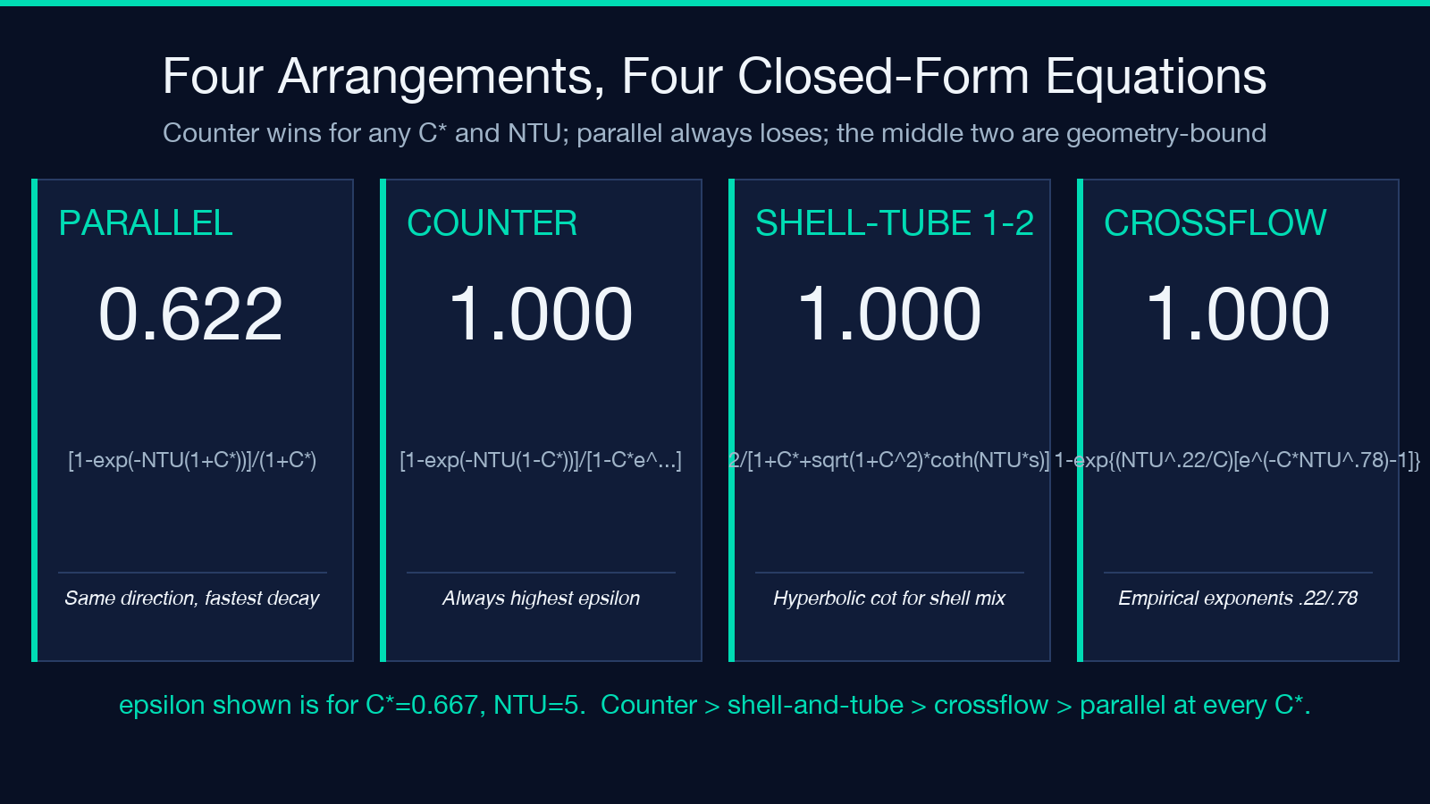
Counter flow inverts the geometry: ε = [1 − exp(−NTU · (1 − C))] / [1 − C · exp(−NTU · (1 − C))]. When C approaches 1, the denominator blows up against the numerator and the formula degenerates; the calculator substitutes the balanced form ε = NTU / (1 + NTU) in that limit, which is the textbook condensation of the balanced counter-flow case. Counter flow is the arrangement that always wins for a given NTU and C*; if you can route the streams against each other, do.
Shell-and-tube one-two pass is the third form and the most algebraically dense: ε = 2 / [1 + C + √(1 + C²) · (1 + exp(−NTU · √(1 + C²))) / (1 − exp(−NTU · √(1 + C²)))]. The expression under the square root — 1 + C*² — is the shell-and-tube geometry factor, and the (1 + exp)/(1 − exp) term is a hyperbolic cotangent that captures the cross-stream mixing in the shell side. For NTU > 3 the exponential terms dominate and the formula collapses toward counter flow; for NTU < 0.5 the formula is closer to a single-pass arrangement with a small correction.
Crossflow both-unmixed is the most numerically delicate: ε = 1 − exp[(NTU^0.22 / C) · (exp(−C · NTU^0.78) − 1)]. The fractional exponents (0.22, 0.78) are empirical constants fitted to the experimental crossflow geometry; they are not derivable from first principles. The C in the denominator makes the formula undefined as C approaches 0, which is the phase-change edge case the calculator handles by collapsing to the parallel-flow formula instead.
Reading the Five Outputs Together
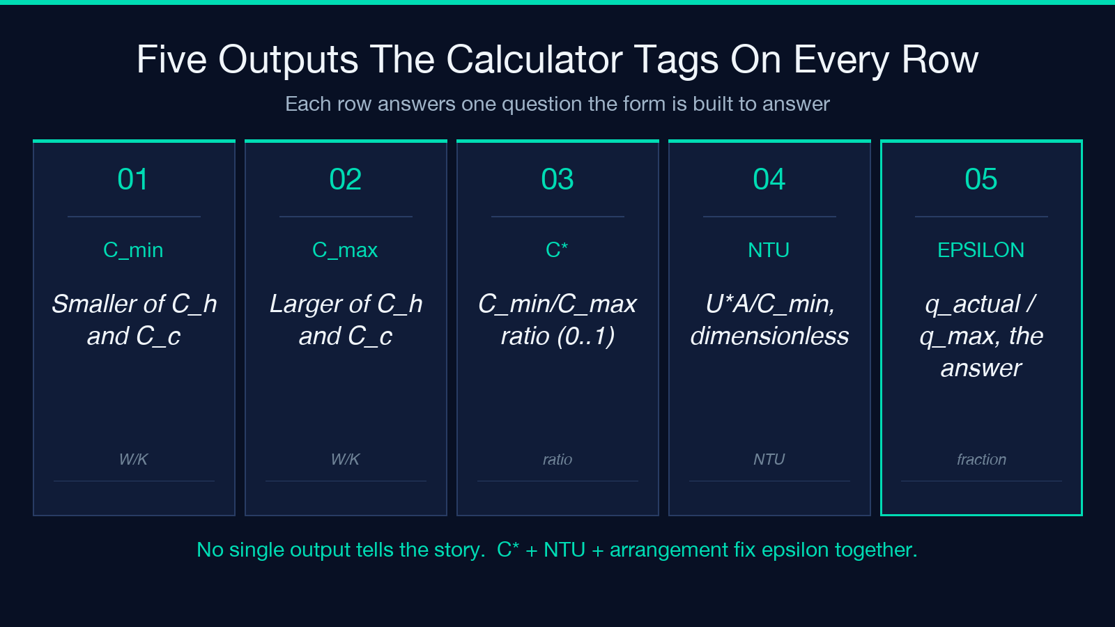
The calculator returns five numbers: ε, NTU, C_min, C_max, and C*. None of them alone tells the full story, and the order in which you read them matters.
C_min and C_max are diagnostic: they confirm which stream the calculator identified as limiting and let you sanity-check the capacity-rate inputs. C is the dimensionless geometry knob, and it is the value you want to log first because every subsequent number depends on it. NTU is the dimensionless heat-transfer knob; it is the product U · A / C_min, and once you know NTU and C the effectiveness is fully determined by the arrangement alone. ε is the headline output and the answer to the rating question: how much of q_max is the exchanger actually moving.
A worked example for the calculator: pick C_h = 1000 W/K, C_c = 1500 W/K, U = 500 W/(m²·K), A = 10 m², arrangement counter. The calculator computes C_min = 1000, C_max = 1500, C = 0.6667, NTU = 5, and ε = 0.928. That 92.8 percent effectiveness means the counter-flow exchanger moves 92.8 percent of the thermodynamic maximum heat rate the boundary conditions allow. For comparison, the same inputs in parallel give ε ≈ 0.622, in shell-and-tube-1-2 give ε ≈ 0.857, and in crossflow-both-unmixed give ε ≈ 0.793. The arrangement ranking — counter > shell-and-tube > crossflow > parallel — holds at every intermediate C, and is the headline reason to choose a counter-flow geometry when the construction budget allows it.
Three Failure Modes the Form Will Silently Accept
Three input errors will produce numerically valid but physically meaningless outputs. The first is a swapped U and A. If you type A = 500 and U = 10, the calculator still computes a valid NTU = U · A / C_min = 5 and a valid ε, but you have just rated a 500-square-meter exchanger with a 10 W/(m²·K) coefficient, which is not a real heat exchanger. The form does not have a sanity range on U because it varies too widely across fluid pairs; the engineer has to confirm U against a heat-transfer handbook for the specific fluid combination before trusting any output.
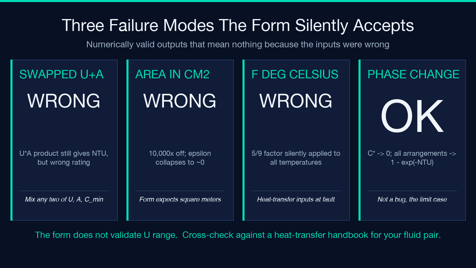
The second is A in square centimeters. The form expects meters and the engineering convention is meters, but if a CAD export or a data sheet hands you area in cm², the calculator will silently rate an exchanger with one ten-thousandth of the intended area. A 100 cm² exchanger with a realistic U will return an ε of essentially 0 because NTU is tiny, and the form has no way to know the unit is wrong. The third is a temperature unit selector flipped from °C to °F without flipping the numeric values. A T_h,in = 120 °F value fed as if it were 120 °C silently changes q_max by a factor of 5/9, and downstream q_actual and the outlet temperatures inherit the error.
When C* = 0 Is the Whole Story
The phase-change edge case — one side boiling or condensing — collapses C* to 0 because the phase change pins the side temperature and gives that stream an effectively infinite capacity rate. In that limit every arrangement formula reduces to ε = 1 − exp(−NTU), regardless of geometry. The intuition is that the dominant stream acts like a constant-temperature reservoir, so the only thing that matters is how fast the smaller stream can deliver heat to it. For NTU = 3, ε = 1 − exp(−3) = 0.95; for NTU = 5, ε = 0.993; for NTU = 10, ε = 0.99995. Phase-change exchangers are almost always effectiveness-limited by the non-phase-change side, and the geometry only matters insofar as it sets NTU.
The corollary is that for a condenser or boiler, the arrangement selector is largely cosmetic: counter, parallel, shell-and-tube, and crossflow all converge to the same ε to within three significant figures once C < 0.05. The calculator’s C output makes that convergence explicit; if it returns C* < 0.01, you can ignore the arrangement and just compute ε = 1 − exp(−NTU) directly.
Optional Inlet Temperatures and the Outlet Branch
When you supply T_h,in and T_c,in in addition to the five required inputs, the calculator extends its output from ε and NTU to q_max, q_actual = ε · q_max, and both outlet temperatures T_h,out and T_c,out. The outlet branch is what makes the calculator usable for rating in both directions: forward rating (given geometry, find q and the outlets) and inverse rating (given a target outlet, find the required area).
The outlet formulas are straightforward energy balances: T_h,out = T_h,in − q / C_h and T_c,out = T_c,in + q / C_c. Note the sign on the cold side: the cold stream gains heat, so its outlet temperature is higher than its inlet. The temperature unit selector governs both inlets and outlets, and the calculator correctly applies the 5/9 factor on Fahrenheit differences but not on Fahrenheit absolute temperatures. A second crossflow worked example: C_h = C_c = 2000 W/K, U = 400, A = 8, T_h,in = 120 °C, T_c,in = 30 °C. The calculator returns C* = 1, NTU = 1.6, ε ≈ 0.667, q_max = 2000 · 90 = 180000 W, q_actual ≈ 120000 W, T_h,out ≈ 60 °C, T_c,out ≈ 90 °C. The 60 K outlet temperature on the hot side and the 60 K rise on the cold side conserve energy exactly, and the gap between hot-side outlet (60 °C) and cold-side outlet (90 °C) is the temperature approach — the smallest temperature difference anywhere in the exchanger, which is the standard check for whether a crossflow geometry can hit a process target.
The Heat Exchanger ε-NTU Calculator handles the four arrangements, the C* collapse, and the optional outlet branch in a single form, but the engineering judgment — what ε is acceptable for the process, what NTU is achievable for the fluid pair, what the temperature approach must be — still lives in the chart and the engineer’s head. For the LMTD-based alternative and the planar heat-flow comparison, see the Cylinder Radial Heat Conduction calculator and the broader heat-transfer library at elysiatools.com/en/tools.
