
Two averaged-element solvers process the same low-Earth orbit and disagree by twelve kilometres per revolution. That gap is not a bug; it is the difference between a model that re-averages the J2 zonal potential every step and one that closes Gauss-equation averaging into a closed-form secular rate. Both are correct within their own assumptions. The danger is treating one as a single-source of truth for mission analysis.
The ESA PB05-Style Brouwer-Lyddane Averaged-Element Orbit Propagator takes the second path. It propagates mean Keplerian elements under the EGM96 zonal harmonics J2 through J6, reconstructs first-order J2 short-period oscillations back into osculating coordinates, and folds in double-averaged luni-solar quadrupole effects for elliptical inclined perturbers. The output is a secular drift curve over a configurable window, a frozen-orbit diagnostic, and a sun-synchronous inclination solve – all on the same report page. Treat the model as a fast lens on long-arc behaviour, not as a stand-in for high-fidelity numerical integration.
Why averaged elements earn their slot in the propagation stack
Numerical RK4 propagators step the Cartesian state vector every integration tick. They are accurate to integration order, but they pay for that accuracy with wall-clock time, and they obscure which forces actually drive long-arc drift. Averaged-element models take the opposite trade: replace the fast Keplerian motion with a slowly varying mean-element state, then reconstruct the fast oscillation only when needed.
The PB05 / Brouwer-Lyddane tradition is the canonical example. You write the disturbing potential (here the EGM96 zonal harmonics) in terms of the classical Keplerian elements, orbit-average over one revolution using the true anomaly, and the secular rates of the mean elements fall out as closed-form expressions of (a, e, i). The Delaunay variables are the natural coordinate system for this averaging because the mean anomaly becomes the fast variable and drops out of the secular equations entirely.
The tool implements this in two ways and cross-checks them. The numerical Gauss-equation averaging path integrates the Gauss planetary equations directly over one orbital period and tabulates the resulting rate as a function of the mean state. The closed-form J2 rates use the classical analytical expressions (RAAN and argument of perigee drift proportional to J2 times cos(i) and J2 times (5 cos-squared(i) – 1)) as a built-in cross-check. When the two agree to better than 1e-8 rad/day over the propagation window, you have a working model; when they disagree, you have a starting point for a debugging session.
The J2 through J6 zonal stack
The EGM96 zonal field is a sum of Legendre harmonics P_n(sin(geocentric latitude)) with coefficients J_n. J2 is the equatorial bulge term and dominates everything below the GNSS altitude band; J3 adds the southern-hemisphere asymmetry that drives frozen-orbit analysis; J4, J5, and J6 contribute smaller secular terms that nevertheless accumulate over multi-year propagations.
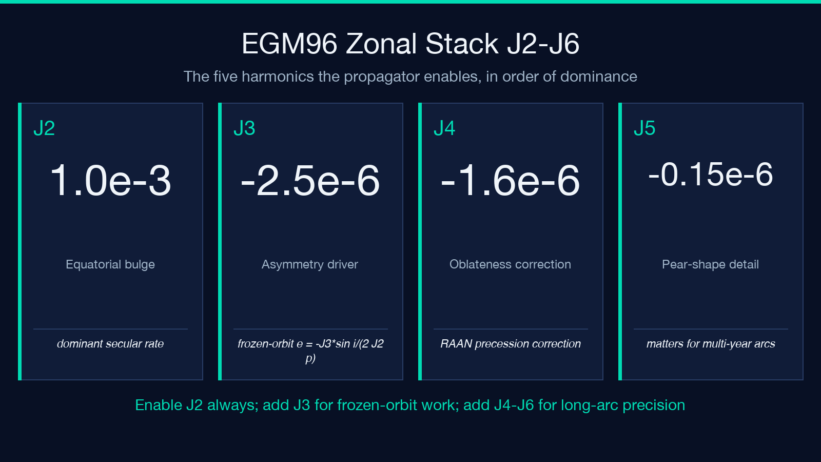
The propagator lets you enable each zonal harmonic independently. Set J2 only and you have the classical Kozai-Izsak Brouwer solution; add J3 and the frozen-orbit condition e = -J3sin(i)/(2J2*p) becomes reachable; add J4 and the secular RAAN rate gains a small but non-negligible correction; J5 and J6 are cosmetic for most low-Earth orbits but matter for precise long-arc comparisons.
A practical debugging pattern: turn off everything except J2, confirm the closed-form RAAN drift matches the numerical Gauss-equation average to better than 1e-10, then enable J3 through J6 in sequence. When the agreement breaks, the last harmonic you enabled is the culprit. This is faster than reading the source line-by-line.
Short-period reconstruction and mean-to-osculating
The averaged-element model gives you the secular drift. To compare against a numerical propagator or a TLE-derived state, you need to reconstruct the short-period J2 oscillation that was averaged away.
The first-order J2 short-period term is the dominant piece. The osculating semi-major axis oscillates by approximately J2(R_earth/a)^2 (1 – 1.5*sin-squared(i)) times the eccentricity vector; the osculating eccentricity and inclination pick up smaller but correlated terms. The propagator’s mean-to-osculating routine applies these corrections analytically – no numerical root-finding, no iteration – so the conversion is essentially free compared to the propagation itself.
A subtlety: the reconstruction is first-order in J2. Higher-order J2 short-period terms exist and matter when you are comparing averaged-element output against high-precision numerical propagation at the metre level. The tool does not pretend otherwise. The in-report RK4 cross-validation panel is the honest answer: if your application needs metre-level agreement, use a numerical propagator.
Luni-solar perturbations and the Kozai-Lidov 39.23-degree critical mutual inclination
For orbits below the GNSS belt, the Sun and Moon exert non-negligible gravitational perturbations that the J2 zonal stack does not capture. The classical treatment is to average the third-body disturbing function over both the satellite’s orbit and the perturber’s orbit (the “double averaging” approximation), which leaves a secular quadrupole term that depends on the mutual inclination between the satellite orbital plane and the perturber orbital plane.
The propagator implements this double-averaged quadrupole for an elliptical inclined perturber – the realistic case for the Moon, whose eccentricity is about 0.05 and whose orbit is inclined about 5 degrees to the ecliptic. The resulting secular equations contain a critical mutual inclination near 39.23 degrees (the Kozai-Lidov critical angle, sometimes given as arccos(sqrt(3/5))). Near and beyond this mutual inclination, the orbit-averaged equations develop a Kozai-Lidov oscillation in eccentricity and argument of perigee that the simple secular model does not capture.
The tool surfaces this explicitly. When the mutual inclination crosses the 39.23-degree threshold, the report flags the regime change and reports the secular rates assuming the linearised quadrupole – a reasonable approximation inside the regime, but a known approximation outside it. For lunar-resonant mission design, this is the boundary you need to be aware of.
Frozen orbits, sun-synchronous orbits, and ground-track resonance
Three canonical orbit classes reduce to closed-form conditions on the secular rates:
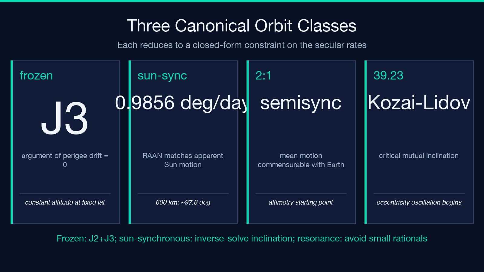
– Frozen orbits: the secular drift of the argument of perigee is zero. The classical J2-J3 frozen-orbit condition is e = -J3sin(i)/(2J2*p), which is what the propagator checks when you enable J3. Frozen orbits are useful for altimetry missions that want a constant altitude at a fixed ground-track latitude.
– Sun-synchronous orbits: the secular RAAN drift matches the apparent mean motion of the Sun (about 0.9856 degrees per day). The propagator solves the inverse problem: given the orbit altitude and eccentricity, what inclination produces a sun-synchronous node regression? For a 600 km circular orbit the answer is about 97.8 degrees; for a 800 km circular orbit it is about 98.6 degrees.
– Ground-track repeat orbits: the secular mean motion times the Earth rotation period produces a rational commensurability. The propagator checks the 1:1 (geosynchronous), 2:1 (semisynchronous), 3:2, 5:2, and small-rational resonances with Earth rotation and reports the closest match. This is the starting point for altimetry mission orbit selection.
All three reduce to the same numerical question: find the classical-element state that satisfies a constraint on the secular rates. The propagator does this in report form rather than as a black-box optimiser.
Tesseral resonance checks for the 1:1, 2:1, 3:2, and 5:2 commensurabilities
Tesseral harmonics (the m is not 0 terms in the spherical-harmonic expansion) are not averaged into the secular equations – they show up as long-period perturbations with period equal to the Earth-rotation period divided by the (l – m) difference.
For orbits whose ground-track repeats a small integer number of times per day, the long-period tesseral perturbation can resonantly couple with the orbital motion and produce secular growth in eccentricity. The 1:1, 2:1, 3:2, and 5:2 commensurabilities are the worst offenders. The propagator reports the closest small-rational commensurability of the mean motion and flags orbits within a configurable tolerance band (default 1e-3) so you do not unknowingly design a mission on top of a resonance.
In-report RK4 cross-validation
Every report includes a side-by-side panel that propagates the same initial conditions with an RK4 numerical integrator. The numerical path is slower (milliseconds per propagation versus microseconds for the analytical mean-element path) but accurate to integration order.
Use the cross-validation panel as a sanity check, not as a truth source. If the two paths diverge by more than the expected first-order J2 short-period correction, the analytical path has a bug; if they agree within the correction, the analytical path is doing what it claims. For metre-level mission work, the numerical path is the truth; for design exploration and trade studies, the analytical path is the workhorse.
Where the propagator stops being the right tool
The PB05 / Brouwer-Lyddane averaged-element model is a secular-rate model. It assumes the disturbing potential is small compared to the central Keplerian potential (J2 is the dominant term, but it is still 1e-3) and that the orbit-averaging step is valid (no close approaches, no resonance locking). When those assumptions break – high-altitude MEO orbits near resonance, very low perigees with significant atmospheric drag, lunar-resonant mutual inclinations in the Kozai-Lidov regime – the analytical model produces qualitatively wrong secular rates.
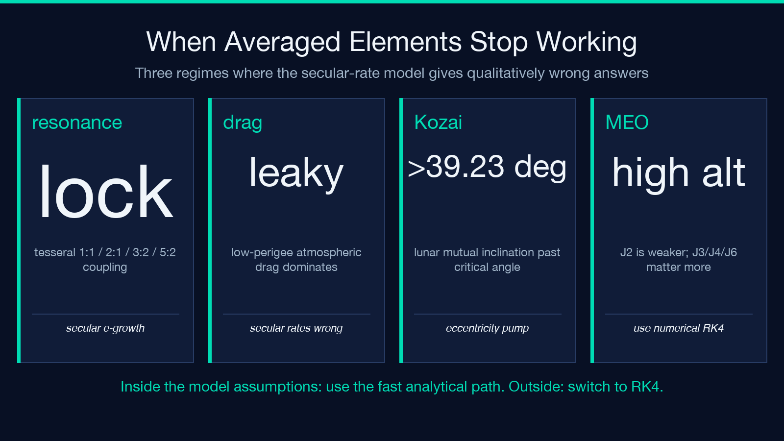
For those cases, switch to the numerical RK4 cross-validation panel as the primary propagation path. Or pull in a higher-fidelity tool. The averaged-element propagator’s job is to be a fast first-look lens on long-arc behaviour, and it does that job well when you stay inside its assumptions.
Explore the ESA PB05-Style Brouwer-Lyddane Orbit Propagator when you need a fast secular-rate model for LEO or GNSS-region design studies, and let the in-report RK4 panel be the honest cross-check.
