Matrix Inverse Calculator Field Guide: When Three Branches of Linear Algebra Decide Whether One Square Matrix Has a Solution

When the linear system A · x = b lands on your screen with a “no unique solution” warning, the question is rarely about whether your algorithm failed — it is whether A⁻¹ exists at all, and that question has three structurally different answers depending on which branch of linear algebra you ask.

A matrix has an inverse if and only if it is square AND its determinant is nonzero — and that is the entire question

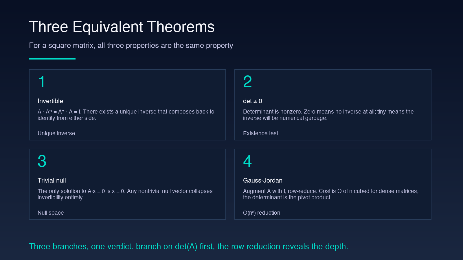
Every property of a matrix that you actually care about for inversion follows from one number: the determinant. Specifically, for an n × n square matrix A over the real numbers, the following three statements are equivalent:

1. A has an inverse A⁻¹ such that A · A⁻¹ = A⁻¹ · A = I.
2. det(A) ≠ 0.
3. The only solution to A · x = 0 is the trivial solution x = 0.

These three are not three separate properties — they are the same property stated three different ways, and the proof uses Gauss-Jordan elimination in about a page. So when a calculator reports “non-invertible” or “determinant is zero,” it is telling you that the matrix fails all three at once, and there is no point looking for some clever workaround that preserves invertibility. Either the determinant is zero or it is not.

The practical question then becomes: how close to zero is close enough to count as “essentially zero” for your purposes? For a 3 × 3 matrix of integers, that threshold is obvious (det = 0 means exactly zero). For a 100 × 100 matrix whose entries come from floating-point sensor data, “det = 1.4 × 10⁻⁸⁵” is technically nonzero but functionally singular — round-off will dominate any inverse you compute. This is where the Matrix Inverse Calculator distinguishes itself: it does not just report the inverse, it reports the determinant, the matrix rank, and the condition number in one pass, so you can see why the answer is what it is.

Branch one: the determinant test for small matrices (n ≤ 4)

For a 2 × 2 or 3 × 3 matrix, the determinant gives you the invertibility verdict and the inverse in essentially the same operation. The Laplace expansion along the first row of a 2 × 2 matrix produces:

| a  b |
| c  d |

with det = ad − bc, and the adjugate formula gives the inverse directly as (1/det) · [[d, −b], [−c, a]]. The exact arithmetic here is why 2 × 2 inverses feel like cheating in linear algebra homework — the answer is always one fraction.

For 3 × 3 matrices, the Sarrus rule extends the same logic to three-by-three without a cofactor expansion, but for anything bigger the cost grows fast. The Laplace expansion of a 4 × 4 determinant has 24 terms of three products each — manageable by hand, painful to debug when one sign is wrong. The calculator does not care about any of this; it switches to Gauss-Jordan elimination as soon as the size permits, and the determinant emerges from the product of the pivots.

This is the “easy” branch — small, well-conditioned, exact arithmetic. The entire diagnostic you need is whether the determinant is zero or not, and what its magnitude tells you about scaling.

Branch two: Gauss-Jordan elimination — and where two failure modes become visible (n ≤ ~100)

Once the matrix passes the size threshold where hand expansion becomes tedious, Gauss-Jordan elimination takes over. The algorithm augments A with the identity I, then row-reduces the augmented matrix to [I | A⁻¹]. The cost is O(n³) for dense matrices, which means a 50 × 50 matrix takes a bit under 60 seconds in pure Python and well under a second in a compiled linear algebra library.

Two failure modes become visible during Gauss-Jordan that the determinant check alone cannot show:

• A zero pivot appears mid-reduction. The current row has no eligible non-zero element in the pivot column, no row swap will find one, and the determinant collapses to zero. This is “structurally singular” — usually a sign of dependent rows or columns in the original matrix.
• A tiny pivot appears mid-reduction. The current row has an eligible pivot, but it is small enough that dividing through multiplies the rounding error by a factor of 1/pivot_size. For a pivot of 10⁻⁶, every subsequent row gets a 10⁶ amplification of round-off. This is “numerically singular” — the determinant is technically nonzero but the computed inverse will be numerical garbage.

The condition number captures exactly this: κ(A) = ‖A‖ · ‖A⁻¹‖. For a well-conditioned matrix, κ is O(1). For an ill-conditioned one, κ can be 10⁶ or 10¹² or larger, and every digit of the inverse past the first few is dominated by round-off regardless of which algorithm you use.

Branch three: the singular value decomposition for matrices you cannot actually invert

For a 1000 × 1000 matrix of sensor data, or any input where the determinant does not fit cleanly into the floating-point range, Gauss-Jordan still works in theory but the practical question shifts. You are no longer asking “is the inverse exact” but rather “what is the best approximate inverse I can compute on the rank-deficient subspace.”

The SVD (A = U · Σ · Vᵀ) splits the matrix into three orthogonal pieces, and the singular values on the diagonal of Σ tell you exactly which subspaces carry signal and which are noise. A “pseudoinverse” A⁺ keeps only the singular values above a chosen threshold and discards the rest — this is what numpy.linalg.pinv does by default at the 1e-15 threshold relative to the largest singular value.

The calculator does not auto-switch to SVD for every input, but the rank report gives you the same information: if rank(A) < n, the matrix is square + singular + rank-deficient, and the inverse either does not exist (when rank is strictly less than n) or is uniquely defined but numerically unstable (when rank equals n but κ is huge). For rectangular inputs (m × n with m ≠ n), the calculator correctly reports “no inverse” — the inverse is a square-matrix concept — and computes the pseudoinverse for users who need the SVD-based least-squares answer.

Reading the three outputs a quality calculator hands you

The output you actually want is not just A⁻¹. The three numbers that decide whether the inverse is trustworthy are:

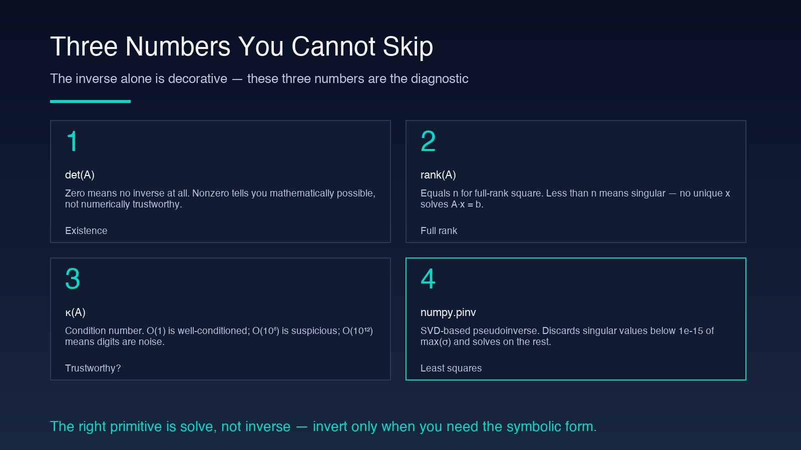
1. det(A) — zero means no inverse at all, nonzero means at least an inverse exists mathematically.
2. rank(A) — equal to n for a full-rank square matrix, less than n means the matrix is singular.
3. κ(A) (condition number) — O(1) is well-conditioned, O(10⁶) is suspicious, O(10¹²) or larger means the inverse is mathematically defined but numerically meaningless.

The Matrix Inverse Calculator surfaces all three in one pass, so the diagnostic and the answer come back together. For a 3 × 3 matrix of small integers, all three are obvious from the determinant alone. For a 50 × 50 matrix from a linear regression or a covariance matrix, the condition number is the only signal that distinguishes “matrix is correct, inverse is correct” from “matrix is correct, inverse is garbage.”

Two worked examples with different failure modes

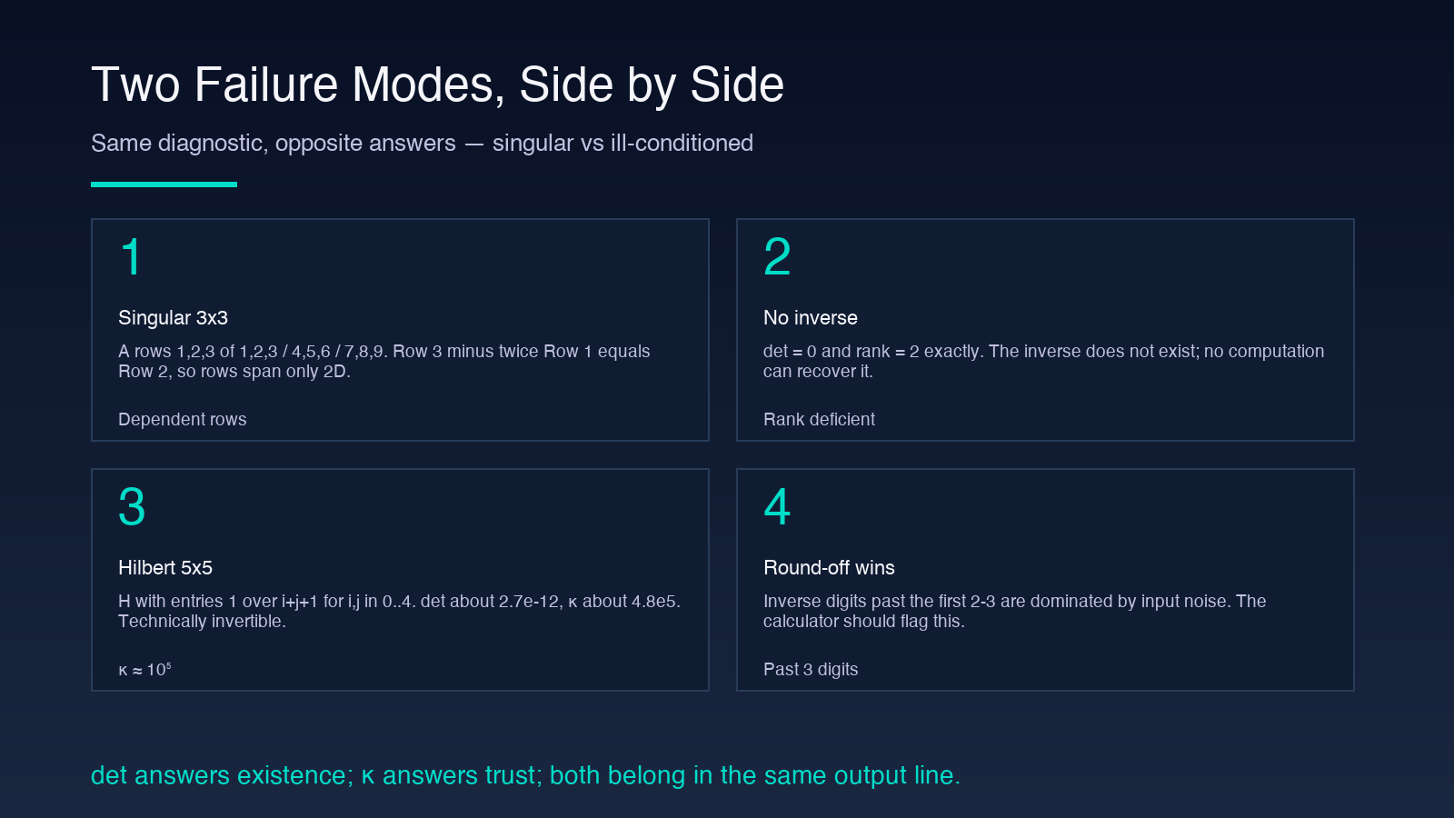
Consider a 3 × 3 matrix built from dependent rows:

A = [[1, 2, 3],
     [4, 5, 6],
     [7, 8, 9]]

Row 3 minus twice Row 1 equals Row 2, so the three rows span only a 2-dimensional subspace. The determinant is exactly 0, rank is 2, and the inverse does not exist. The calculator reports this in one line and refuses to fabricate a result.

Consider instead a Hilbert matrix H with H[i][j] = 1 / (i + j + 1) for i, j in 0..n−1. For n = 5, the determinant is about 2.7 × 10⁻¹² and the condition number is around 4.8 × 10⁵. The matrix is technically invertible, the determinant is technically nonzero, but the inverse grows so fast that round-off in the input data destroys all but the first 2-3 digits of the computed inverse. This is the canonical “ill-conditioned” failure — the calculator should still return an inverse, but flag it visually so you do not trust the trailing digits.

When the answer the calculator gives back is the wrong answer to ask

There is a recurring mistake that shows up in every linear algebra forum on the internet: computing the inverse when you actually wanted to solve A · x = b. The inverse is O(n³) memory and O(n³) work for an n × n matrix. The triangular solve is O(n²) memory and O(n²) work for the same answer. For n = 1000, the inverse requires 8 GB of RAM and roughly a billion floating-point operations; the solve requires 8 KB and a million floating-point operations.

If your real question is “what x satisfies this linear system,” the right primitive is LU decomposition with forward-backward substitution, not matrix inversion. The calculator offers both, but the inverse should be your fallback for symbolic inspection (A⁻¹ of a 2 × 2 writes the closed form naturally) or for diagnosis (the inverse reveals which rows/columns are determinants), not your default solver.

Closing

The three branches of linear algebra — direct for small matrices, Gauss-Jordan for medium, SVD-pseudoinverse for numerically unstable inputs — converge on a single operational rule: trust the inverse only when the determinant is meaningfully nonzero and the condition number is bounded. Every other output from a matrix inverse calculator is decoration around that rule.

If you want to see the failure modes side by side, the Matrix Inverse Calculator runs a singular matrix, a Hilbert matrix, and an identity matrix through the same diagnostic stack and prints the determinant, the rank, and the condition number alongside the inverse. The math behind those three numbers is identical to what any compiled linear algebra library does internally — the difference is that you can see all of them at once.

For more tools that translate raw matrix input into inspectable numerical output, the Elysia Tools collection catalogs the full set.