
A pedigree probability tree is one of those quiet physics-chemistry crossover tools that nobody remembers until they need it: a classroom teacher trying to figure out whether two CF carriers in a row should panic, a genetic-counseling student double-checking a homework answer, or a textbook author trying to put real numbers behind a Mendelian “1/4” diagram. Most online explanations stop at the rule-of-thumb fraction. The work is making that fraction survive the per-parent, per-child branching that real offspring risk actually lives in.
This field guide walks the way the Pedigree Probability Tree handles three concrete inheritance scenarios — autosomal recessive with both parents known carriers, autosomal dominant with one or both parents heterozygous, and X-linked recessive with a carrier mother. Each case gets the same treatment: parental genotype probabilities upstream, per-sex branches downstream, then product rule along the tree and sum rule across the branches the family actually wants.
Why One Fraction Per Inheritance Pattern Isn’t Enough
Textbook genetics compresses an autosomal recessive cross into “1/4 affected, 1/2 carrier, 1/4 unaffected” the moment both parents are known heterozygotes. That is true — but it is also the most optimistic case in real family trees. Before either parent is a known carrier, the relevant probability is the population carrier frequency filtered by any family history on each side. The pedigree tree plugin refactors the calculation into two layers: (1) the probability each parent is a carrier at all, given what we already know about their parents and siblings, and (2) the conditional offspring distribution once those parental probabilities are set. The combined tree carries both.
This two-layer framing is the practical reason most autosomal recessive risk calculators give answers that surprise patients — they bake the second layer in but quietly assume the first. The Pedigree Probability Tree keeps both branches visible so the user can swap the carrier-frequency input and watch the offspring distribution shift.
Autosomal Recessive: Two Known Carriers Make the 1/4 Case
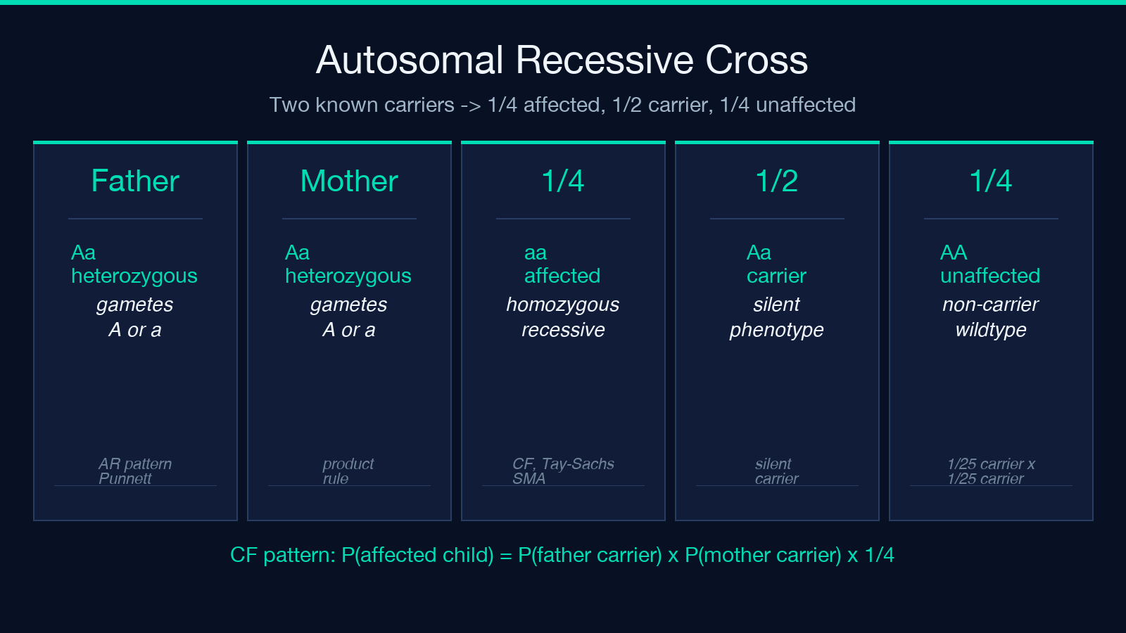
The cleanest pedigree in the dataset is two known heterozygous parents — a father who was tested because his sibling had an affected child, a mother who was tested during prenatal planning. Each produces a gamete pool of half carrier allele, half wild-type. The Punnett square collapses to three genotypes per child: 1/4 homozygous affected, 1/2 heterozygous carrier, 1/4 homozygous unaffected.
The tree plugin shows this as one parental genotype node per parent, each branching into two gametes, then four offspring genotypes with the 1/4 / 1/2 / 1/4 weights explicit. The sum rule across branches gives the same answer as the Punnett square, but the tree format scales — when you ask “given the second child is unaffected, what is the probability the third is affected?”, the tree lets you condition on the previous branch and recover 1/4 by symmetry (each pregnancy is independent).
In clinic, the cystic-fibrosis pattern — delta-F508 homozygous — is the textbook case. CF carrier frequency in Northern-European populations is around 1/25, which gives an at-birth incidence near 1/2500 — the product of two carrier probabilities and one quarter transmission. The plugin exposes both inputs as a single “population carrier frequency” field so the same arithmetic holds for Tay-Sachs (1/30 in Ashkenazi populations), spinal muscular atrophy (1/40 to 1/50), and the rarer metabolic disorders that don’t get general-public screening.
Autosomal Dominant: The 3/4 Trap When Both Parents Are Affected
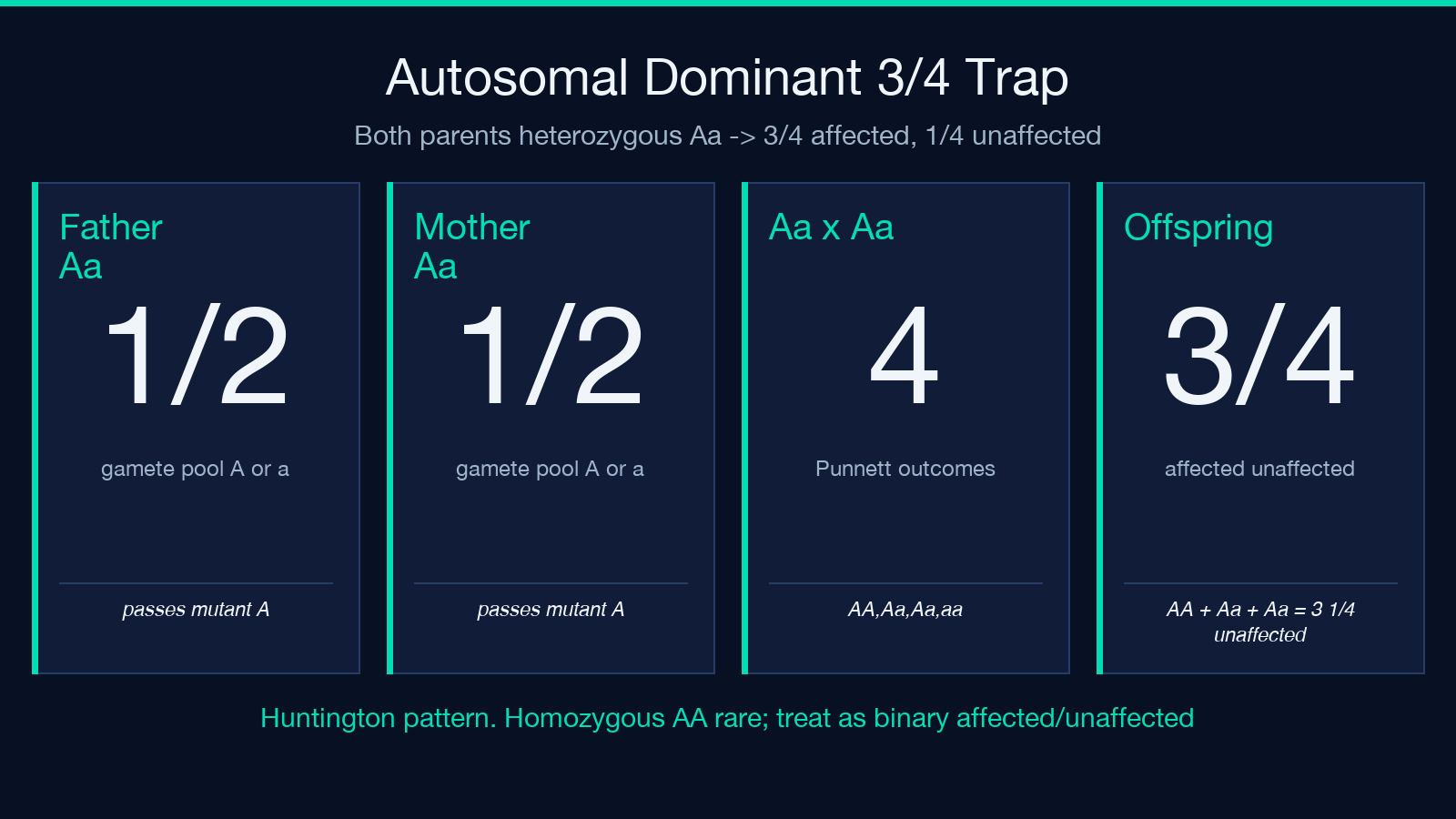
The dominant pattern looks simpler on the surface — affected parent, unaffected child, 1/2 risk. The complication hits when both parents are heterozygous affected. Under the affected-dominant convention, each parent is Aa (heterozygous; homozygous dominant disease alleles are usually embryonic lethal or extremely rare). The offspring distribution becomes 1/4 AA (affected, severe), 1/2 Aa (affected, mild-to-moderate), 1/4 aa (unaffected) — which simplifies to 3/4 affected, 1/4 unaffected when severity is collapsed into a single affected/unaffected binary.
That 3/4 ratio is the Huntington-disease pattern. If a heterozygous parent has a 50% chance of passing the dominant allele, and the other parent is also a known heterozygous patient, the unaffected-child probability drops from 1/2 (one affected parent) to 1/4 (both parents affected). The tree plugin makes this visible by drawing two parental genotype nodes that overlap and the four-leaf offspring tree.
The clinical twist is that “affected” in autosomal dominant diseases often has variable expressivity — the same Aa genotype produces a spectrum from late-onset mild to juvenile-onset severe. The plugin does not try to capture expressivity; the affected/unaffected binary is the calculation the Mendelian framework supports.
X-Linked Recessive: The Per-Sex Branch That Complicates Everything
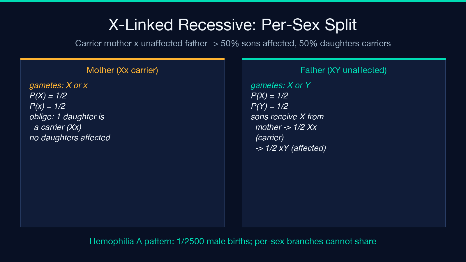
The X-linked recessive case is the place most textbooks wave their hands. The simplest pedigree is a heterozygous carrier mother and an unaffected father. Sons get the mother’s X chromosome with 50% probability: 50% of sons are affected, 50% are unaffected. Daughters get one X from the mother (50% carrier, 50% non-carrier) and a Y from the father: 0% of daughters are affected, but 50% of daughters are carriers. The per-sex branch needs to be drawn separately, because the “50% carrier daughter” outcome does not exist on the son side.
The hemophilia A pattern (factor VIII deficiency) and the Duchenne muscular dystrophy pattern are the textbook cases. Carrier frequencies for hemophilia A are around 1/5000 female births; the family-history multiplier is enormous — a mother with one affected son and one affected maternal uncle has a much higher carrier probability than the population baseline.
The tree plugin handles the per-sex split by drawing two leaf branches under the offspring node: a son-leaf with the X-linked outcomes and a daughter-leaf with the carrier/unaffected outcomes. The overall-child probability is then weighted by the 50% male / 50% female prior.
When Carrier Status Is Unknown: The Bayesian First Layer
The 1/4, 3/4, and per-sex splits above are all second-layer calculations — they assume parental genotype. The first layer is the probability each parent is a carrier at all, given only their family history. A father with two unaffected parents and no affected siblings has the population carrier frequency as his prior. A father with one affected sibling has a much higher prior — specifically, 2/3, because the affected sibling rules out the father being homozygous unaffected, leaving either carrier or unaffected (with carrier probability 2/3 conditional on having at least one carrier parent in the parental cross).
The pedigree tree lets users override the population prior and watch the second-layer numbers shift. Cystic fibrosis gives a good demonstration: the at-birth incidence for a couple with one known carrier and one untested partner is 1/4 × 1/25 = 1/200 instead of the 1/2500 population number — a twelve-fold increase that matches clinical intuition.
Limitations of Tree-Based Calculation
Mendelian tree methods assume complete penetrance, no de novo mutations, and no mosaicism. For the textbook autosomal-dominant, autosomal-recessive, and X-linked-recessive patterns the tree is exact; for everything else the answer needs a clinician and a genetic test.
Where the Mendelian Tree Stops Working
The Mendelian framework misses the trinucleotide-repeat disorders where parent-of-origin effects matter (Fragile X, myotonic dystrophy), the imprinting disorders (Prader-Willi, Angelman), and the mitochondrial inheritance patterns that go through the mother only. These patterns each carry their own branching structure that the autosomal-dominant/recessive/X-linked-recessive tree does not encode.
Another limit is the binary “affected / unaffected” outcome. Many dominant disorders express as a continuous severity score; the tree compresses that distribution into a single bit. Tools that report expected severity (polygenic risk scores, multifactorial inheritance) live in different territory entirely.
Putting It Together: A Worked Example
A couple comes in for prenatal counseling. The father has an affected brother with cystic fibrosis; his parents are both unaffected obligate carriers. The mother has no family history. Plug into the tree plugin: father’s carrier probability = 2/3 (one affected sibling, parents obligate carriers); mother’s carrier probability = 1/25 (Ashkenazi baseline, say). The cross produces affected children at 2/3 × 1/25 × 1/4 = 1/150 — close to the population allele-frequency numerator but elevated by the family history.
The same couple re-runs the calculation once they get a confirmed-negative carrier test for the mother: the affected-child probability collapses to zero for that specific mutation. The tree is recomputable on the fly, which is the practical reason to use a tool rather than memorize a fraction.
If you only remember one thing from this guide: a Mendelian probability tree is two layers, not one. The first layer is parental carrier probability (population frequency, possibly updated by family history); the second is the offspring distribution given those parental probabilities. The Pedigree Probability Tree keeps both layers visible, lets you change the carrier prior, and shows the per-sex branches when X-linked inheritance is the pattern.
It will not replace a genetic counselor, a CF carrier test, or a prenatal diagnostic — but it will tell you what the rules of Mendelian inheritance actually predict, given the inputs you have. That is a useful number to bring into the conversation.
Explore more tools at elysiatools.com.
