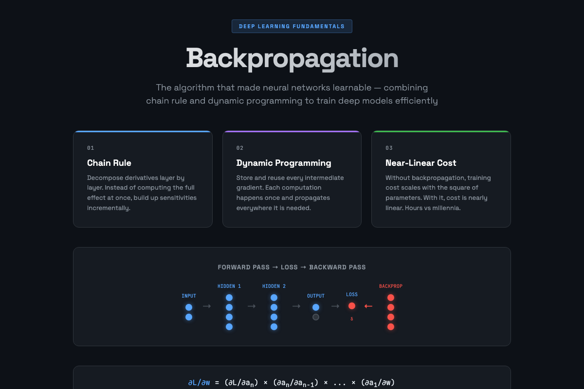
The Algorithm That Made Deep Learning Possible: Understanding Backpropagation
In 1986, three researchers published a paper that most people outside machine learning have never heard of. It did not invent neural networks — those existed already. What it solved was the training problem that had stalled the field for nearly two decades. Without that insight, the AI revolution we are living through today would not exist.
That insight was backpropagation.
Why Neural Networks Stalled for 20 Years
Training a neural network means adjusting millions or billions of numerical parameters so that a function maps inputs to correct outputs. The naive approach — trying every possible combination — fails for the same reason brute-forcing a dictionary fails: the search space is incomprehensibly large.
Gradient descent is better: compute how sensitive the final error is to each parameter, then adjust each one in the direction that reduces error. But computing that sensitivity directly in a deep network is astronomically expensive. Each parameter’s effect on the final output depends on every other parameter between it and the output.
Backpropagation changes this.
The Two Ideas Behind Backpropagation
Backpropagation combines two concepts that existed before 1986: the chain rule from calculus, and dynamic programming.
The chain rule lets you decompose derivatives of composed functions. If y = f(g(x)), then dy/dx = (dy/du) × (du/dx). This lets you build up derivatives layer by layer instead of computing the full effect all at once.
Dynamic programming is about reusing intermediate results. Instead of recomputing the same partial derivatives multiple times, you compute them once and store them. Every gradient in a deep network is computed once and reused everywhere it is needed.
The result is efficiency. Training a neural network should cost roughly as much as the square of the number of parameters. Backpropagation reduces this to near-linear cost. That is the difference between training a model in hours versus millennia.
The Algorithm in Six Steps
The procedure is concrete:
1. Run a forward pass to compute the predicted output y_hat from the input
2. Compute the loss L(y_hat, y) — how wrong the prediction was
3. Compute delta at the output layer — how sensitive the loss is to each output neuron
4. Propagate those deltas backward through the network using the chain rule, computing sensitivity at each hidden layer
5. Compute gradients dW and db for each weight and bias, then update all parameters
6. Repeat until the loss stops decreasing
Steps 3 and 4 are where the algorithm earns its name. Once you have delta at one layer, you can compute delta at the previous layer using only local information — the weights connecting the two layers and the activation function at the current layer. That locality is what makes the whole thing tractable.
The Vanishing Gradient Problem
For years after 1986, deep networks still struggled to train. The issue was subtle: as gradients propagate backward through many layers, they get multiplied together repeatedly. If the average local derivative is less than 1, the gradient shrinks exponentially — gradient vanishing. If it is greater than 1, the gradient grows exponentially — gradient explosion.
In the vanishing case, early layers learn almost nothing. In the exploding case, parameters oscillate wildly. Both make training deep networks unreliable, which is why early neural networks were shallow — two or three layers was all anyone could reliably train.
Geoffrey Hinton has called this “the lotka-volterra problem” in hindsight, referring to how predator-prey population oscillations constrain ecosystem depth. The practical fix — residual connections — did not arrive until 2015 with ResNet. But by then, practitioners had developed a toolkit of partial solutions that made moderate depth workable.
Modern training relies on several complementary techniques. ReLU and GELU activations keep gradients flowing by avoiding saturation. He initialization preserves variance across layers. BatchNorm and LayerNorm add learned scaling that keeps signals in a stable range. Residual connections let gradients skip layers entirely. AdamW with warmup and cosine decay provides reliable optimization. Gradient clipping prevents explosion during early training. Mixed precision (fp16 or bf16) accelerates training without meaningfully affecting convergence.
The Invisible Backbone
When people discuss AI breakthroughs, they cite transformers, attention mechanisms, and large-scale pre-training. Backpropagation is invisible in these conversations — it is assumed, not celebrated.
But without it, none of those other advances would be trainable at scale. Backpropagation is the mechanism that assigns credit and blame to a billion parameters simultaneously. Without it, deep learning remains a theoretical possibility, not an engineering reality.
The three researchers who formalized it — David Rumelhart, Geoffrey Hinton, and Ronald Williams — solved the credit assignment problem. They did not invent neural networks. They made them learnable. Every chatbot, every image generator, every speech recognizer running in production today inherits that solution.
Explore the Backpropagation Deep Dive visualization to walk through forward and backward passes step by step, experiment with gradient stability across different network depths, and see chain rule multiplication produce vanishing or exploding gradients in real time.