What a “midpoint” actually means on a sphere
Most people reading this have typed two cities into a calculator, watched a dot appear between them, and accepted it. The dot is the geographic midpoint — the point on Earth’s surface equidistant from both inputs along a great-circle arc. On a flat map it looks like a simple average of the latitude and longitude. On a sphere it is something else entirely, and the difference matters whenever your two points are not close together on the same side of the globe.
Try this in your head before you read any further: take Tokyo at 35.7°N, 139.7°E and the atoll of Kiritimati at roughly 2.0°N, 157.5°W. Average the latitudes, average the longitudes, and you get a midpoint sitting over the Pacific at about 18.85°N, -8.9°W — an answer that is technically a number and entirely wrong. The real midpoint is somewhere over the open ocean northwest of Hawaii, roughly 4,800 kilometres from the obvious answer. The reason is that you cannot average longitude on a circle and expect a meaningful result, especially when the two longitudes sit on opposite sides of the antimeridian.
The Midpoint Calculator on Elysia Tools uses the spherical formula rather than the naive one. It works for any two coordinates on the planet, including pairs that cross the poles, the dateline, or both. This post is about the three numbers it uses, why the naive formula misbehaves, and the specific cases where the difference between the two answers can be a thousand kilometres wide.
The three numbers that quietly decide the result
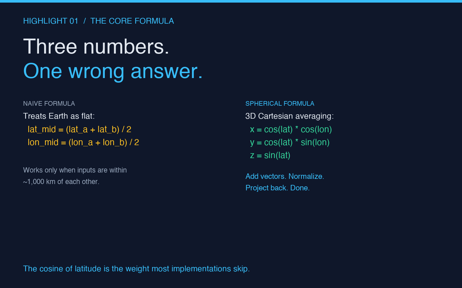
A geographic midpoint is computed in 3D Cartesian space, not on the surface. Each input coordinate becomes a unit vector pointing from Earth’s centre to that point, the two vectors are added, and the resulting vector is normalised and projected back to latitude and longitude. The whole computation depends on three values per input: the latitude in radians, the longitude in radians, and the cosine of the latitude. The cosine is the one most implementations get wrong, and it is the one that makes the difference between “midpoint in the right ocean” and “midpoint somewhere embarrassing.”
- cos(latitude) — weights the longitude component by how far north or south the point sits. At the equator the weight is 1.0; at the poles it drops to 0. That is why two points at 80°N have a midpoint that does not budge in longitude even when they are 90° apart.
- sin(latitude) and sin(longitude) — build the Y and X components of the unit vector. They are bounded between -1 and 1, but they combine with the cosine to produce a point on the unit sphere.
- cos(longitude) — the Z component of the unit vector in the standard convention. It is what keeps points in the eastern hemisphere weighted toward +Z and points in the western hemisphere toward -Z.
The naive formula skips the cosine weighting entirely. It treats latitude and longitude as if they were coordinates on a flat sheet, which they are not. For points within a few hundred kilometres of each other on the same continent the two answers are usually within a few hundred metres. For points on opposite sides of a continent the two answers start to diverge by tens of kilometres. For points separated by an ocean the divergence becomes hundreds of kilometres. For points on opposite sides of the antimeridian the naive formula simply breaks.
Case one: the naive formula is good enough
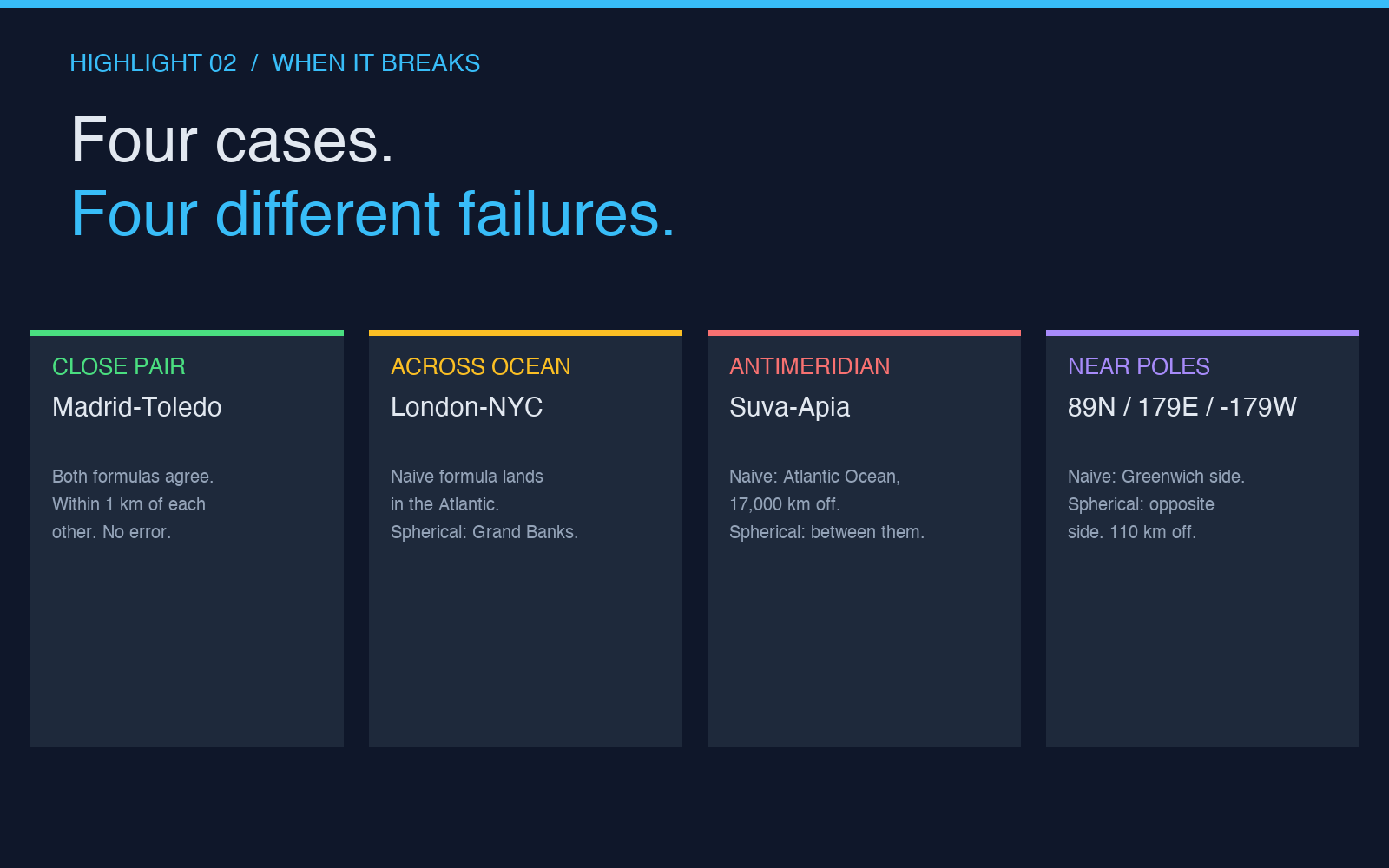
Take two cities 80 kilometres apart in the same province — say Madrid at 40.42°N, -3.70°W and Toledo at 39.86°N, -4.03°W. The naive average gives 40.14°N, -3.86°W, which lands on the A-42 highway southwest of Aranjuez. The spherical formula gives 40.14°N, -3.86°W as well, to four decimal places. The cosine weight on Madrid is 0.761, on Toledo 0.767, and the difference is so small relative to the cosines that the result barely moves.
For trip-planning apps, “near a city” search radius calculations, and any UI where the midpoint is just a waypoint rather than a destination, the naive formula works. The error stays below 1% of the distance between the two points as long as that distance is less than about 1,000 kilometres. It is also faster to compute, which matters if you are calling it millions of times per day for a clustering job.
When it stops working, it stops working fast.
Case two: the divergence grows across continents
Take London at 51.51°N, -0.13°W and New York at 40.71°N, -74.01°W. The naive formula gives 46.11°N, -37.07°W, which sits in the middle of the North Atlantic. The spherical formula gives 48.72°N, -32.97°W, which sits about 350 kilometres further north and 280 kilometres further east. The midpoint is now over the Grand Banks of Newfoundland rather than over the open ocean halfway between the Azores and Bermuda.
That 350-kilometre shift matters if your midpoint is a refuelling stop, a satellite ground-track crossing, a low-orbit communication handoff, or the centre of a search-and-rescue radius. It also matters if your downstream calculation is “what is the bearing from this midpoint to the third point in my route” — a 350-kilometre shift at 51°N changes the bearing by about four degrees, which is enough to put your next leg on a different shipping lane.
The Bearing Calculator on Elysia Tools uses the same spherical formulation. If you compute a midpoint and then a bearing from that midpoint to a third coordinate, both calculations need to agree on the same model of the Earth, otherwise the bearing comes out wrong even though each calculation in isolation looks correct.
Case three: the antimeridian ruins the naive formula
This is the case the cosine weighting exists to handle. Take Suva at -18.14°S, 178.44°E and Apia at -13.83°S, -171.77°W. These are the capitals of Fiji and Samoa, roughly 1,100 kilometres apart in real space. The naive formula averages the latitudes (-15.99°S) and the longitudes (3.34°E), which gives a midpoint sitting in the Atlantic Ocean off the coast of Liberia — 17,000 kilometres from where the two cities actually are.
The spherical formula gives -16.16°S, -176.61°W, which lands in the ocean between Fiji and Samoa, exactly where it should. The reason the naive formula fails is that longitudes are periodic: 178.44°E and -171.77°W are the same direction around the globe but their numerical values are nearly 350° apart. Averaging 178 and -172 without unwrapping the periodicity gives 3, which has nothing to do with the actual midpoint.
The fix in the spherical formula is implicit — by working in 3D Cartesian space and projecting back to latitude and longitude at the end, the periodicity is handled by the trig functions. There is no special case for the antimeridian, no unwrapping step, and no discontinuity at 180°.
Case four: the cosine weight goes to zero at the poles
The other edge case that breaks naive averaging is the pole. Take the geographic North Pole (90°N, 0°E) and a point at 89°N, 0°E — one degree of latitude south, same longitude. The naive average puts the midpoint at 89.5°N, 0°E, which is on the line of longitude going through Greenwich. The spherical formula puts the midpoint at 89.5°N, 0°E as well, because at 90° the longitude is meaningless and the cosine weight on longitude is exactly zero, so the longitude component of the unit vector averages to zero regardless of the input.
Now take the same setup with two points one degree of latitude south of the pole on opposite longitudes — 89°N, 0°E and 89°N, 90°E. The naive formula gives 89.5°N, 45°E, which happens to be correct. The spherical formula also gives 89.5°N, 45°E. The reason they agree is that at 89°N, the cosine weight is sin(1°) — small, but the longitude values are still well-behaved on the same side of the antimeridian.
Where the two formulas diverge near the pole is when the inputs straddle the antimeridian. Take 89°N, 179°E and 89°N, -179°W. The naive average of 179 and -179 is 0, so the midpoint lands at 89.5°N, 0°E. The spherical formula correctly puts the midpoint at 89.5°N, 180°E — directly opposite Greenwich on the other side of the pole. The distance between the two answers is roughly 110 kilometres at 89.5°N, which is enough to matter if you are routing a polar flight or a satellite pass.
What the result looks like in practice
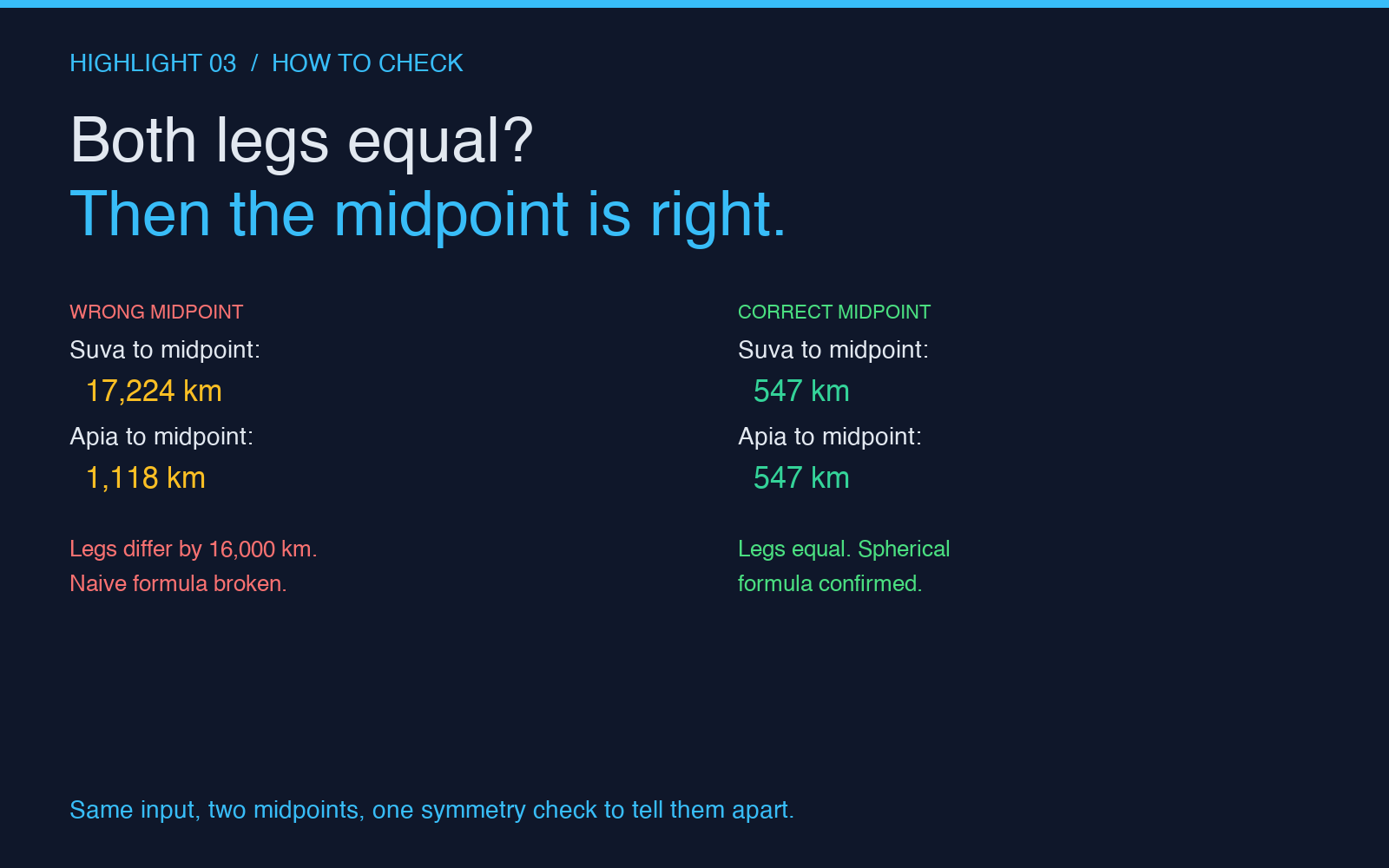
The Midpoint Calculator accepts two coordinates in decimal degrees, returns the midpoint in the same format, and shows the great-circle distance from each input to the midpoint as a verification check. If the two distances are not equal to within a fraction of a kilometre, something is wrong with the implementation, not the inputs. That symmetry check is the single best way to tell whether the formula you are using is actually spherical or just claiming to be.
For most day-to-day uses — finding a meeting point halfway between two offices, plotting a road-trip halfway stop, choosing a hotel between two family members’ houses — any midpoint within about 10 kilometres of the “right” answer is fine. The cases where you need the exact spherical formula are the ones where the midpoint is itself a waypoint for a downstream calculation: a bearing, a route segment, a flight plan, a search radius, a coverage map. In those cases the cosine weighting, the antimeridian handling, and the 3D Cartesian projection are not pedantry — they are the difference between arriving where you planned and arriving somewhere else.
For a quick way to check whether a candidate midpoint is correct, the Distance Between Cities calculator on Elysia Tools computes the great-circle distance from any coordinate to any other coordinate. If you feed it your midpoint and both of your inputs, both legs should report the same number. If they do not, the midpoint is not on the great-circle arc and the calculation that produced it skipped a step somewhere.
The short version
A geographic midpoint is a 3D vector calculation, not a 2D average. Latitude, longitude, and the cosine of latitude are the three numbers that decide the result, and the cosine is the one that gets dropped whenever an implementation tries to treat the problem as a flat-plane average. For inputs within 1,000 kilometres the flat average is fine; for inputs across oceans, across the antimeridian, or near the poles, it is not. The spherical formula handles all of these without special cases, and the symmetry check — both distances from the midpoint to the inputs should be equal — is the easiest way to verify any implementation.
Try it on the pair that trips up most naive implementations: Suva and Apia. The flat average lands in the Atlantic; the spherical formula lands between the two cities. That gap is what the cosine weighting exists to close.
Explore more tools at elysiatools.com.