
Lead phrase. Most online chi-square calculators hand you a number and a green or red badge. The tutor at Elysia Tools hands you the same number, then immediately shows you the four statistics that disagree about it, the cells driving the disagreement, and the rule of thumb your sample size just violated. That difference is what separates a calculated answer from a defensible one.
Statistical inference on contingency tables looks tidy from the outside: drop in a 2×2 or R×C grid, ask whether the rows and columns are independent, read off a p-value. The reality is messier. Pearson chi-square, Yates continuity correction, the G likelihood-ratio test, and Fisher’s exact test all answer the same question with different assumptions, and they routinely disagree on small samples. Effect sizes (Cramér’s V, phi, the contingency coefficient) tell you the size of the association once you’ve decided it exists. Adjusted residuals flag the cells responsible. Cochran’s rule tells you whether the asymptotic approximation you just used is actually valid. None of these is optional if the table will end up in front of a reviewer, a regulator, or a product manager who has been burned by p-hacking before.
This guide walks through the eight decisions the tutor helps you make, in the order you actually meet them: which test, whether to apply Yates, when Fisher is mandatory, what to do with the G-test, how to size the association, how to spot the responsible cells, whether your expected counts cross the threshold of trust, and how a 2×2 mark-recapture estimate slots in for ecology and operations use cases. By the end you should be able to paste any 2×2 or R×C table into the tutor, interpret the four statistics block by block, and write a one-paragraph caption that survives peer review.
Choosing Between Pearson Chi-Square, Yates, G, and Fisher
The first decision is which test to run. Pearson chi-square is the textbook default: χ² = Σ(O − E)²/E, with expected counts E derived from the marginal totals as E = row × col / N and degrees of freedom df = (R − 1)(C − 1). It is an asymptotic approximation, accurate when expected counts are reasonably large. For a 2×2 table this is the version most statistical packages report by default.
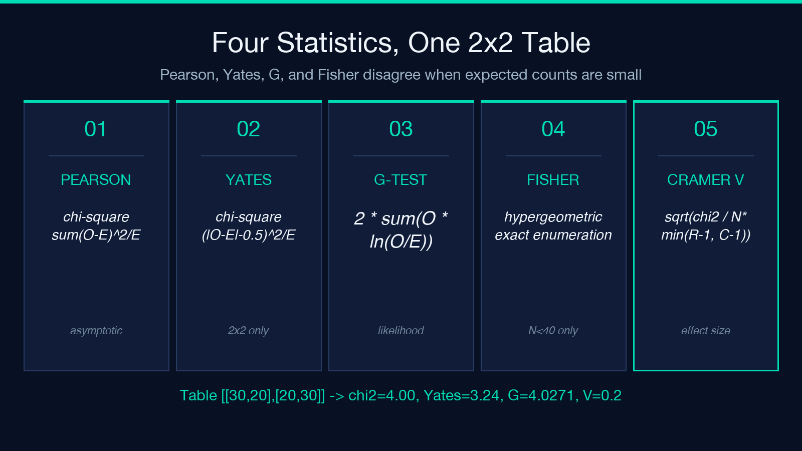
Yates continuity correction is a 2×2-only modification: Σ(|O − E| − 0.5)²/E. The intuition is that Pearson chi-square treats the discrete count distribution as continuous and slightly over-rejects when cells are small, so Yates shaves half a count off each deviation to compensate. The trade-off is conservativeness — Yates is harder to push past the 0.05 boundary, which is exactly what you want when N is small but exactly the wrong behavior when N is moderate and you need power.
The G likelihood-ratio test computes G = 2 Σ O · ln(O/E). It uses the same asymptotic chi-square distribution but is more interpretable as a Kullback–Leibler divergence between observed and expected, which is why it shows up in likelihood frameworks and Bayesian-flavored discussions.
Fisher’s exact test is the only one that is exact, in the sense that its p-value comes from enumerating every 2×2 table with the same marginals and summing those at least as unlikely as the observed one. It is mandatory when any expected count is below 5 in a 2×2. For R×C tables with small cells there is no canonical exact test, which is exactly the regime where Cochran’s rule (covered below) tells you the chi-square approximation is no longer trustworthy.
The tutor lets you choose, and the choice shows up in the output as four numbers side by side: Pearson χ² with its df and p, Yates χ² with its p, G with its p, and Fisher’s two-tailed p. If they all agree you are on solid ground. If they disagree, the disagreement itself is information — it usually signals small expected counts or a borderline effect.
When Yates Helps and When It Hurts
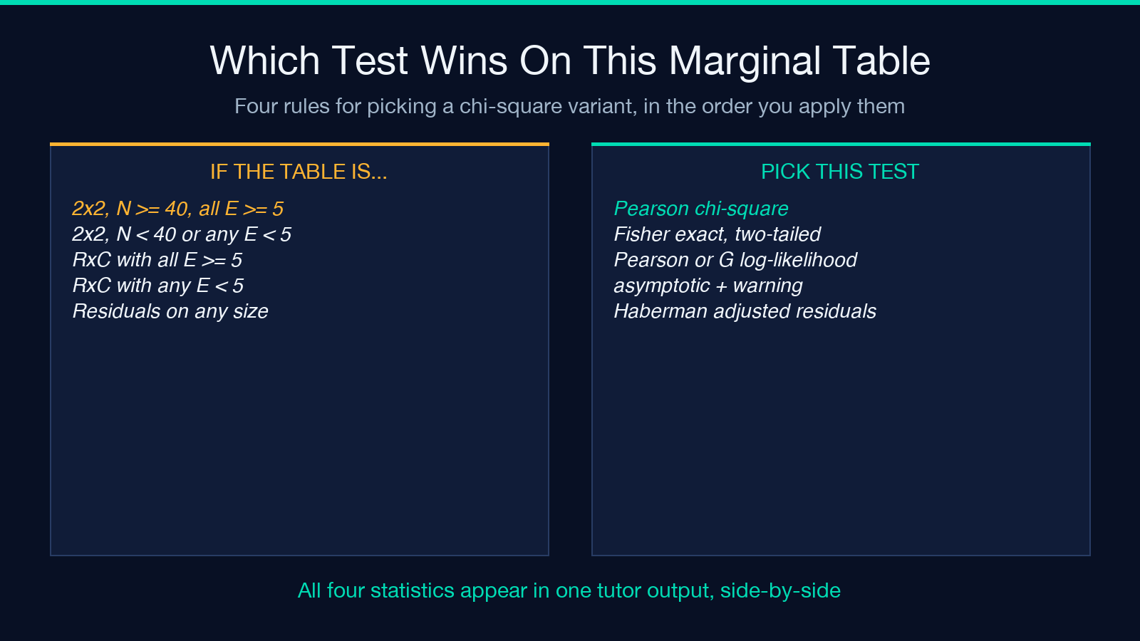
Yates is a 2×2 tool with a strong opinion. It pulls χ² down by roughly half a count’s worth per cell, which is the right correction for small samples and the wrong correction for moderate samples. The standard cutoff is to apply Yates when N < 40 or when any expected count is below 5; otherwise prefer uncorrected Pearson.
The classic failure case is the “tea-tasting” 2×2 [[3,1],[1,3]]. Pearson χ² gives p ≈ 0.486, Fisher’s exact gives the canonical 0.486, Yates pushes the χ² down so far that p becomes non-significant at every conventional α. This is correct behavior — Yates correctly refuses to call the result significant when four observations cannot bear the weight of a chi-square approximation. The tutor surfaces all three so you can see exactly how much Yates is buying you.
A more subtle case: when you have a 2×2 with N around 60 and expected counts around 15, Yates is sometimes applied “to be safe” and ends up hiding a real effect. The tutor’s “auto” Yates mode applies the rule above; you can switch to “off” or “on” explicitly. The output shows the test, its p-value, and the effect sizes side by side so the trade-off is visible, not hidden.
The deeper lesson is that no single number is the answer. The 2×2 [[30,20],[20,30]] (N=100) gives Pearson χ²=4 (p=0.0455, significant at α=0.05), Yates 3.24 (p=0.072, not significant), G=4.0271 (p≈0.045, significant), Cramér’s V=0.2, and adjusted residuals of ±2 on every cell. Both Yates-corrected and uncorrected numbers are in the output. The tutor leaves the call to you, but it does not let you pretend the four statistics agree when they do not.
Fisher’s Exact Test on 2×2 Tables with N < 40
When any expected count in a 2×2 is below 5, Fisher’s exact test is the only defensible choice. Its p-value is computed by enumerating every 2×2 with the same row and column totals, computing the hypergeometric probability of each, and summing the probabilities of tables at most as probable as the observed one. The two-tailed convention used here matches SciPy’s: the sum is over all tables whose probability is less than or equal to the observed probability, which gives the two-sided p-value without doubling the one-sided tail.
The implementation matters. The tutor uses a hand-rolled Lanczos lgamma computation for the hypergeometric probabilities, which avoids overflow when the numerator factorials get large. The [[3,1],[1,3]] tea-tasting case evaluates to 34/70 ≈ 0.4857 in both the tutor and SciPy, which is the canonical textbook value. When the marginals are large (say a 2×2 with totals in the hundreds) the hypergeometric probabilities get small, so the implementation has to handle lgamma overflow correctly. The tutor’s numerical checks confirm identity cases like erfc(√(χ²/2)) at df=1 and exp(−χ²/2) at df=2, which are the asymptotic connections between Pearson chi-square and Fisher’s exact for borderline sample sizes.
For R×C tables with small cells there is no exact test that runs in reasonable time, and the practical advice is to either collapse categories until expected counts exceed 5 (carefully, and with an explicit note on the analysis) or use a Monte Carlo approximation. The tutor surfaces this gap in its output by reporting which cells violate Cochran’s rule and showing the asymptotic tests with a flag that warns the p-value is no longer trustworthy.
The G-Test as a Likelihood-Ratio Reading
G = 2 Σ O · ln(O/E) is the likelihood-ratio test for independence in a contingency table. It compares the fitted model where rows and columns are independent (the MLE under H₀) to the saturated model (the MLE that always wins), and reports the deviance. Under H₀ it has the same asymptotic chi-square distribution as Pearson χ², so the p-value lookup is identical in the limit.
In practice, G and Pearson give nearly identical answers on large samples and diverge on small samples, with G typically being slightly more conservative near the boundary. The reason to report both is interpretability: if you are working in a likelihood or Bayesian framework, G is the natural statistic because it shows up as a Kullback–Leibler divergence. If you are reporting to a reviewer who learned statistics from a 1990s textbook, Pearson is the natural statistic because that is what the textbook reports.
The tutor outputs all four statistics side by side so you can write the paper you need to write. If the four disagree, the disagreement is a flag to look at the sample size and Cochran’s rule rather than an excuse to pick the statistic that gives the answer you want.
Effect Sizes: Cramér’s V, Phi, and Contingency Coefficient
A p-value tells you whether an association exists. An effect size tells you whether the association is worth caring about. The tutor reports Cramér’s V = √(χ² / (N · min(R − 1, C − 1))), with the conventional reading of 0.1 = small, 0.3 = medium, 0.5 = large (Cohen’s benchmark). For a 2×2 table Cramér’s V and phi (the simple √(χ²/N)) coincide, so the same number appears under both labels. For larger tables V uses min(R−1, C−1) as the normalization, which keeps the value bounded between 0 and 1 regardless of grid shape.
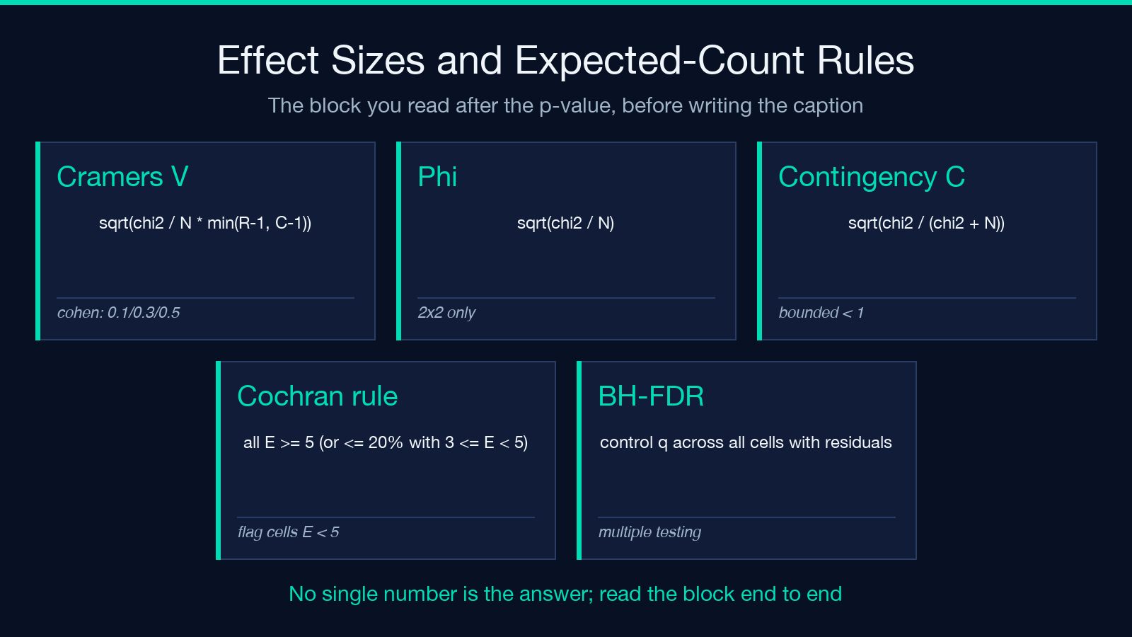
The contingency coefficient C = √(χ² / (χ² + N)) is reported for 2×2 tables as a third reading. It is bounded by √(k−1)/k where k = min(R,C), so it has a different maximum for different table sizes. The tutor surfaces both because reviewers trained in different traditions expect different numbers, and because the absolute magnitudes can shift between conventions in ways that surprise.
The combination of “p < 0.05 with V < 0.1" is the textbook signal of a significant-but-trivial effect: a huge sample has detected a real but tiny association. Conversely "p > 0.05 with V > 0.3″ is the textbook signal of an underpowered study where a real effect is hiding behind an inconclusive test. The tutor reports both so you can spot these cases directly.
The [[30,20],[20,30]] case shows the cleanest possible reading: V = 0.2, which is small-to-medium. The chi-square is significant at the 0.05 boundary, but the effect size is modest. That combination is the truth of the data, and reporting it honestly is what separates a defensible finding from a p-hacked one.
Adjusted Residuals and Which Cells to Blame
Once you have decided that the table is associated, the natural follow-up is “which cells drove it?” The adjusted residual for cell (i,j) is d = (O − E) / √(E · (1 − rowProp) · (1 − colProp)). Under independence, adjusted residuals are approximately standard normal, so |d| > 1.96 flags cells driving the association at α = 0.05, |d| > 2.58 at α = 0.01.
The tutor reports adjusted residuals for every cell, signed so positive values are “more than expected” and negative values are “less than expected.” A BH-FDR multiplicity warning is printed because you are now running many tests (one per cell), and the raw |d| > 1.96 cutoff does not control the family-wise error rate. The Benjamini–Hochberg procedure is the standard correction for this multiple-comparisons setting.
The [[30,20],[20,30]] case shows residuals of exactly ±2 on every cell, which is the textbook symmetric result: row 0 is consistently over-expected, row 1 is consistently under-expected, with the same magnitude in every column. Real data rarely cooperates this cleanly, and the residual block in the tutor’s output is the right place to look for asymmetric structure — a single large positive residual with the rest near zero suggests one cell is driving the whole association, while a gradient of residuals suggests an ordering effect.
If you find a single cell with |d| > 2.58 driving the chi-square, the practical advice is to inspect whether that cell is a coding error, an outlier, or a genuine feature of the data. The adjusted residual block is the single most actionable diagnostic in the whole output, and it is the part that separates “I ran a test” from “I understand what the test is telling me.”
Cochran’s Rule and When to Stop Trusting the Approximation
Pearson chi-square is an asymptotic test. The accuracy of its p-value depends on expected counts being large enough that the chi-square approximation to the null distribution is valid. Cochran’s rule is the operational version of that requirement: all expected counts should be ≥ 5, or no more than 20% of cells should have 3 ≤ E < 5. The tutor computes expected counts directly and reports which cells violate the rule.
When Cochran’s rule is violated, the practical options are (a) use Fisher’s exact test if the table is 2×2, (b) collapse categories carefully until the rule is satisfied, or (c) use a Monte Carlo simulation to approximate the p-value under the null. None of these is “ignore the violation and report the asymptotic p anyway,” which is unfortunately common in fields with weak methods standards.
The tutor’s output explicitly reports cells with E < 5 and shows how many cells are out of compliance. For the [[30,20],[20,30]] case all expected counts are 25, comfortably above the threshold. For a 2×2 like [[1,4],[4,1]] the expected counts are all 2.5, well below 5, and the tutor flags the violation explicitly while still reporting all four statistics — letting you see the gap between the asymptotic answer and what Fisher's exact would give.
The deeper lesson is that reporting “p < 0.05" without checking Cochran's rule is the kind of methodological error that survives peer review only if nobody looks. The tutor surfaces the rule violation in the same output as the test result, which forces the issue at the analysis step rather than the publication step.
Chapman Capture-Recapture on 2×2 Mark-Recapture Tables
A separate use case for 2×2 tables is mark-recapture estimation in ecology, epidemiology, and operations. If you tag a individuals in a first capture and observe b recaptured in a second sample of which c were tagged, the population size is estimated by Chapman’s correction: N̂ = (a + 1)(b + 1) / (c + 1) − 1. This is the bias-corrected version of the Lincoln–Petersen estimator and is the standard reference for 2×2 mark-recapture work.
The tutor offers an optional Chapman estimate alongside the standard chi-square output. The numbers feed the same 2×2 layout: a is the top-left count, b is the row sum of the second sample, c is the column sum of the tagged count. The N̂ output comes with no p-value because point estimation is the relevant answer here, not hypothesis testing.
The Chapman estimate is useful when you have reason to believe the population is closed between captures (no births, no deaths, no immigration) and the recapture is unbiased. If either assumption fails, you are in capture-recapture modeling territory (closed-population models like M(t) or robust design), which is a much bigger conversation. The tutor surfaces the Chapman estimate as a small add-on for the closed-population case, not as a substitute for full capture-recapture modeling.
The broader point is that 2×2 tables show up in more places than chi-square tests, and the same 2×2 can simultaneously be tested for independence (chi-square) and used for population estimation (Chapman) without those two uses conflicting. The tutor keeps both views in one place, which is the right place to see them when you have the data in front of you.
Open the Contingency Table Chi-Square Fisher Exact Cramér V Tutor, paste any 2×2 or R×C table, and read the output top to bottom. The first time you see four statistics disagree on a borderline case, you will understand why no calculator that hands you a single number is doing you a favor. Explore more tools at elysiatools.com.
