When Two Notes Become One: The Hidden Geometry of Beat Frequency
Strike two tuning forks — one at 440 Hz, one at 442 Hz — and listen. What you hear is not two pitches but a single note pulsing twice per second. That wobbling “wah-wah-wah” is beat frequency, and it is one of the most useful phenomena in all of acoustics.
The Moment Two Waves Collide
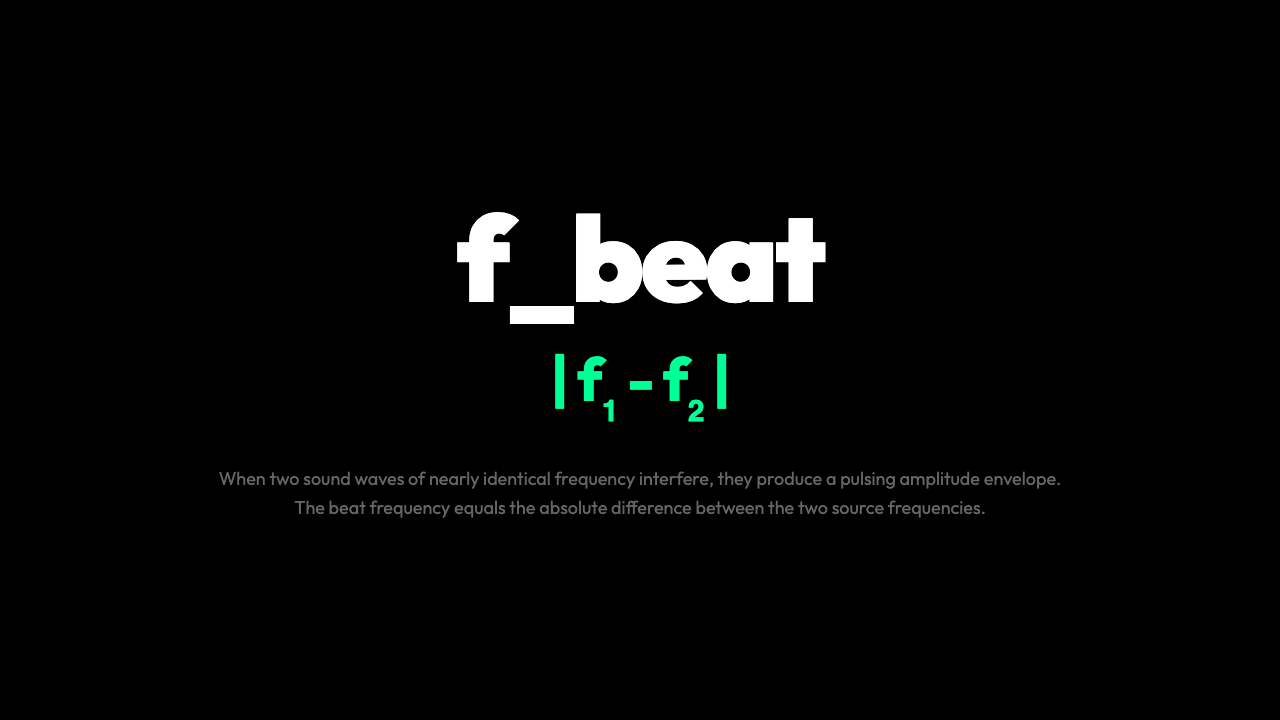
Sound waves are pressure oscillations. When two waves of nearly identical frequency occupy the same space, they do not pass through each other harmlessly. They interfere. Periodically they sum to a large displacement (constructive interference); periodically they cancel (destructive interference). The result is an amplitude envelope that rises and falls at the difference frequency.
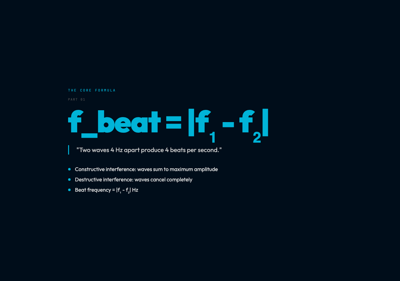
This is the beat frequency formula:
f_beat = |f₁ – f₂|
Two waves 4 Hz apart produce 4 beats per second. Two waves 30 Hz apart produce a noticeable roughness, almost a chord. Two waves 1 Hz apart produce a slow, almost physical throb.
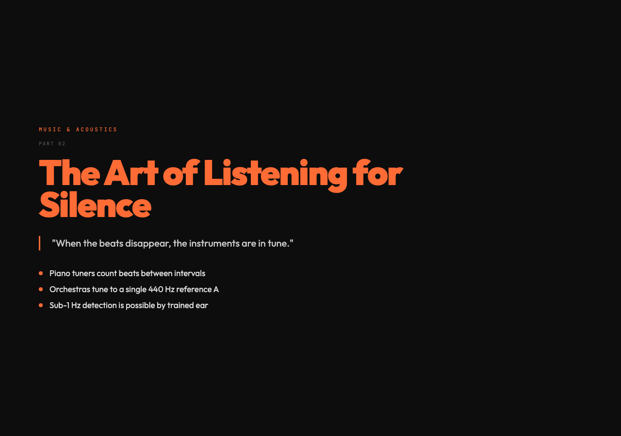
The phenomenon is so intuitive to trained musicians that most learn to ignore the two original pitches entirely and listen only to the beats themselves. When the beats disappear, the instrument is in tune.
Why Musicians Were the First Beat Scientists
Piano tuners have used beat frequency for over two centuries. The procedure is elegant: play your reference tone, then play the same note on the instrument. If beats slow down, the instrument is converging on the reference. When the beats are gone, the interval is pure.
For a piano technician working across the full88-key range, this is not trivial. The temperament problem — dividing the octave so that all keys sound equally in tune — requires counting beats between specific intervals in different octaves. A fifth might beat 3 times per second when slightly flat. A major third might beat 10 times per second when sharp. The entire keyboard’s tuning map is built from these beat relationships.
The same principle applies to orchestral tuning. Before a performance, the oboe plays a 440 Hz A. Every musician listens for their instrument’s relationship to that note, counting beats as the difference between two nearly-identified pitches.
The Math Behind the Wobble
If wave 1 is y₁ = sin(2πf₁t) and wave 2 is y₂ = sin(2πf₂t), their sum uses the identity:
sin A + sin B = 2 sin(π(f₁+f₂)t) × cos(π(f₁-f₂)t)
The first factor is a high-frequency carrier at the average frequency. The second factor is a low-frequency modulator — the envelope. That envelope oscillates at (f₁ – f₂)/2, which corresponds to beats occurring at |f₁ – f₂| per second. The math is clean and direct, a product of trigonometric addition formulas taught in any high school trigonometry class.
The same math appears in AM radio, where a carrier wave is multiplied by an audio signal to “ride” the carrier. Interference and modulation are cousins.
Four Domains Where Beats Matter
Instrument Tuning
This is the oldest and most tactile application. A violin string tuned to 442 Hz against a 440 Hz reference produces a 2 Hz beat — slow enough to count accurately. Experienced tuners can detect sub-1 Hz differences by feel and ear combined.
Doppler Radar
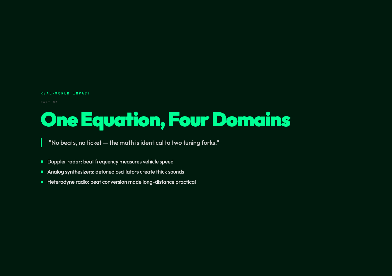
Police radar guns transmit a continuous microwave signal at a known frequency. The signal bounces off your car and returns at a slightly shifted frequency due to the Doppler effect. The police receiver mixes the transmitted and received signals and listens for the beat frequency. That beat frequency is directly proportional to your velocity. No beats, no ticket. The math is the same as two tuning forks — only the wavelength has changed.
Synthesizer Design
Detuning two oscillators slightly and mixing them is one of the oldest synthesizer techniques. The resulting thick, chorused sound is the acoustic signature of 1980s analog synthesizers. The Roland Juno, the Minimoog, and most hardware modular synths use this principle. The beating creates the perception of a larger, more complex sound than a single oscillator could produce.
Heterodyne Radio Reception
Early radio receivers worked by mixing an incoming high-frequency signal with a locally generated signal. The resulting beat frequency was lower — often in the audible range — where it could be amplified and heard. This “heterodyne” principle is why old radios had that characteristic tunable whistle between stations. The mathematics of beat frequency made long-distance radio communication practical decades before digital signal processing.
What Happens When Beats Disappear
The most striking moment in beat frequency is when f₁ = f₂ exactly. The beat frequency becomes zero. The two waves are perfectly synchronized — always in phase, always reinforcing. The amplitude is constant. The wobble stops.
This is the in-tune moment. But it also reveals something deeper: the two original frequencies are still there. They have not merged. They have synchronized. The beats are not a third sound — they are the relationship between two sounds. What disappears is the modulation, not the underlying waves.
This is why beating is so informative. A beat frequency of 0 Hz tells you that f₁ and f₂ are identical to within a tiny fraction of a Hz. No other acoustic test gives you that precision without electronic measurement.
The Threshold Where Beats Become a New Note
At around 15 beats per second, something shifts. Individual beats become difficult to distinguish. Instead, you begin to hear a new, lower pitch — the difference tone. Two tones at 440 Hz and 460 Hz stop sounding like “wah-wah-wah” and start sounding like a steady low note at 20 Hz.
This is the liminal zone between rhythm and pitch. Below 15 Hz, you perceive discrete pulses. Above it, the beats fuse into a continuous tonal sensation. The brain reorganizes the information, switching from a temporal pattern to a spectral one.
The Ear as a Spectrum Analyzer turns out to be not quite accurate. The ear is a time-frequency analyzer, and the beat frequency region reveals where the transition between those two modes lives.
Try It Yourself
The visualization lets you adjust two frequencies independently and watch the combined waveform change in real time. You can set up slow beats (2 Hz), moderate beats (4 Hz), or fast beats (8 Hz). The tuning fork preset gives you the classic 440 + 442 Hz combination that musicians use daily.
Pay attention to the combined waveform — it is not a flat oscillation but a modulated carrier wave. The envelope is the beat frequency made visible. In the live audio output, the same phenomenon is audible as amplitude pulsation.
What makes beat frequency remarkable is its universality. The same mathematics governs a piano tuner counting beats, a police officer measuring your speed, and a synthesizer programmer layering detuned oscillators. It is one phenomenon, four domains, and the same equation every time.