
Five tests, one tutor, and a table that decides whether your chi-square is even legal. When you feed a 2×2 grid into the Contingency Table Chi-Square Fisher Exact Cramér V Tutor, the tool walks the table through Pearson chi-square, Yates-corrected chi-square, the G likelihood-ratio test, Fisher’s exact hypergeometric, and three effect-size measures (phi, Cramér’s V, contingency coefficient), then flags every cell whose expected count is below Cochran’s rule, applies Haberman adjusted residuals with BH-FDR multiplicity correction, and for 2×2 mark-recapture tables prints a Chapman estimator on top. The seven decisions buried in that pipeline — which test to run, whether to apply Yates, when Fisher replaces chi-square, how to interpret Cramér’s V, how to read an adjusted residual, when to accept a result with a flagged cell, and whether Chapman is even on-topic — decide whether your categorical analysis lands as a defensible statistic or as a number you have to apologize for later. This field guide walks through the seven decision points, the three traps (chi-square on sparse cells, V reported as a percentage, raw residuals without multiplicity correction), and the one configuration question that changes everything: are any expected counts below 5.
What the Tutor Actually Computes
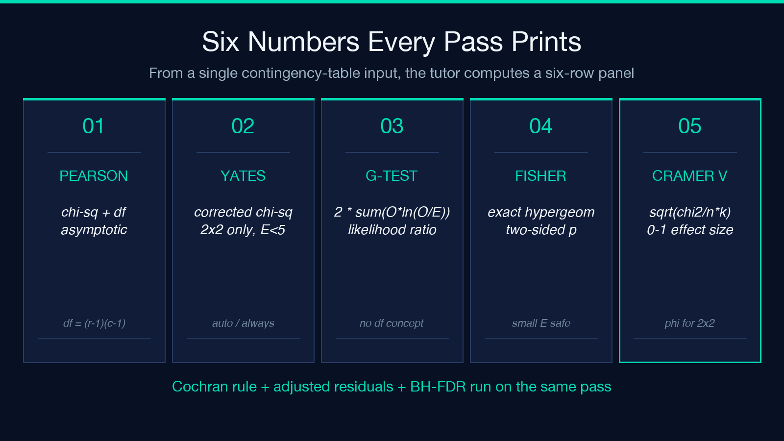
The tutor accepts a contingency table as rows-on-lines, cells-comma-or-whitespace-separated, with no header row. Paste "30, 20n20, 30" and the engine parses it into a 2×2 matrix, computes row and column marginals, then derives six numbers per pass: Pearson chi-square with degrees of freedom (rows-1)*(cols-1), Yates continuity-corrected chi-square (only on 2×2, only when any expected count is below 5 by default), the G likelihood-ratio statistic 2 * sum(O * ln(O/E)), Fisher’s exact two-sided p-value via a hand-rolled hypergeometric with lgamma (no R dependency), Cramér’s V for general R×C, and phi for the 2×2 case. On the same pass it computes Haberman adjusted residuals (O - E) / sqrt(V) where V is the cell-level variance from the inverse of the expected-count table, applies Benjamini-Hochberg FDR correction across all cells, and tags any cell whose adjusted residual exceeds the BH critical value. A separate pass runs Cochran’s rule — “no expected count should be below 1, and no more than 20 percent of expected counts should be below 5” — and emits a yellow warning when either threshold trips. For 2×2 mark-recapture inputs (cells representing caught-not-caught, recaptured-not-recaptured), the tutor also prints a Chapman estimator (M+1)(C+1)/(R+1) - 1 with a 95 percent CI derived from the Poisson approximation.
The Seven Decision Points
The pipeline looks automated but every step has a judgment call.
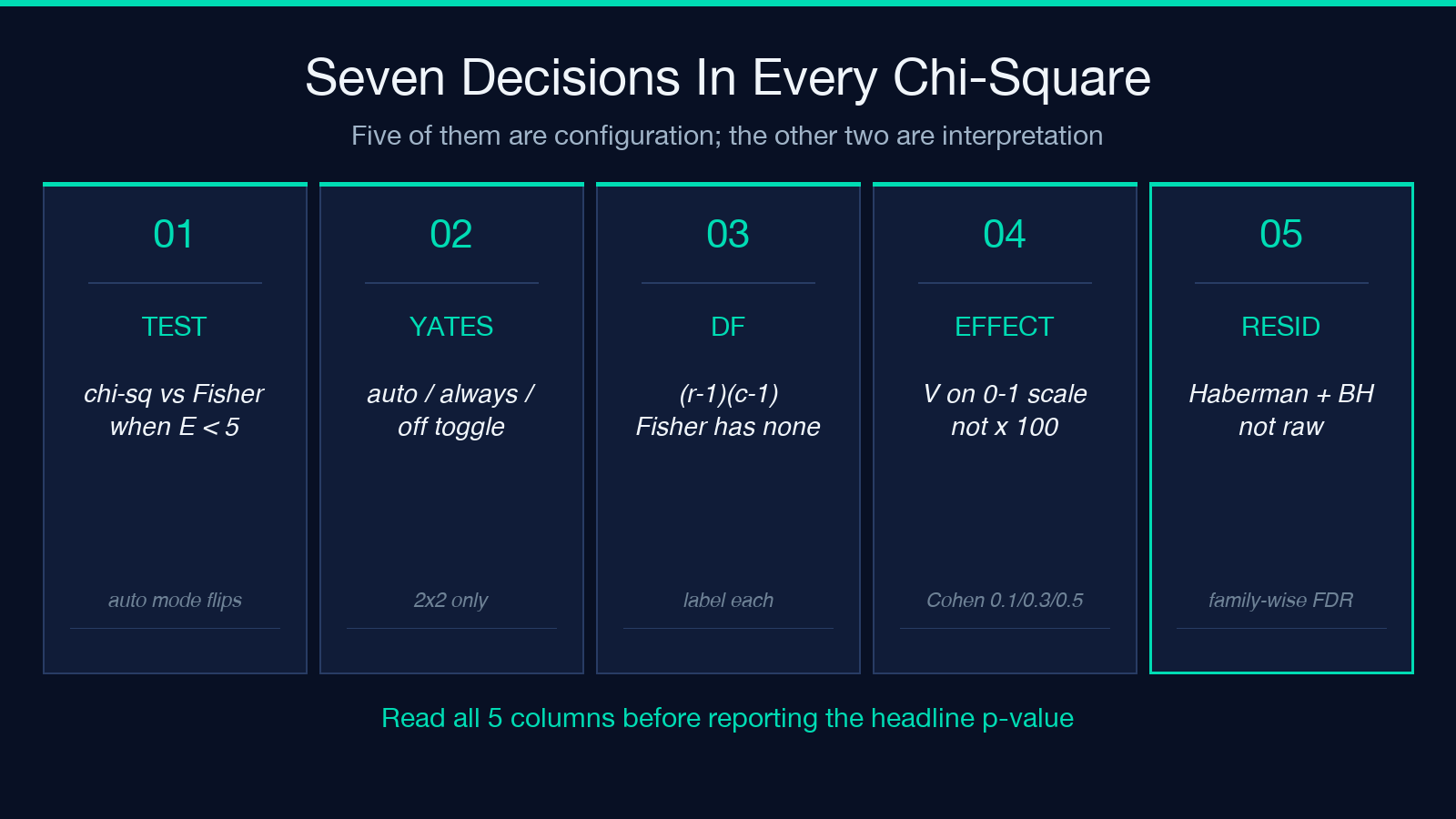
1. Test selection — Pearson chi-square vs Fisher’s exact. When any expected count is below 5, Pearson chi-square’s asymptotic distribution is unreliable; Fisher’s exact (two-sided, computed via the hypergeometric sum over all tables at least as extreme) is exact for any sample size. The tutor’s auto mode flips to Fisher whenever Cochran’s rule trips; always forces Pearson regardless (useful for teaching, dangerous for reporting).
2. Yates continuity correction. Applied by default only on 2×2 with at least one E < 5. Yates shrinks the chi-square numerator by 0.5 before squaring to approximate Fisher’s discrete distribution. Modern statistics textbooks increasingly discourage Yates on computational grounds — Fisher’s exact is exact, Yates is an approximation — but the tutor still computes it because some downstream software expects the number.
3. Degrees of freedom. (rows-1)*(cols-1) for chi-square, but Fisher’s exact is always two-sided and has no df in the classical sense. Reporting both side-by-side is fine if you label them.
4. Effect size — Cramér’s V vs phi. Phi is just Cramér’s V for 2×2: sqrt(chi2 / n). For R×C, V generalizes with min(rows-1, cols-1) in the denominator. Cohen’s benchmarks are rough: 0.1 small, 0.3 medium, 0.5 large. Reporting V as a percentage (V x 100) is a common error — V is a unitless proportion.
5. Adjusted residuals and BH-FDR. A raw residual (O - E) / sqrt(E) is misleading when you have many cells because 5 percent will exceed 1.96 by chance alone. Haberman’s adjusted residual divides by the cell-level variance (from the inverse of the expected-count table) and the tutor applies BH-FDR so that the family-wise false discovery rate stays controlled. A cell flagged significant after BH is the unit you report.
6. Cochran’s rule. Two thresholds: every expected count above 1, and no more than 20 percent of cells below 5. Either tripping means chi-square is no longer trustworthy. The tutor computes expected counts and prints the offending cells; you decide whether to switch to Fisher, collapse categories, or collect more data.
7. Chapman estimator — only for 2×2 mark-recapture. Chapman (M+1)(C+1)/(R+1) - 1 corrects the Lincoln-Petersen bias when sample sizes are small. If your 2×2 is “exposed/diseased” rather than “marked/recaptured”, Chapman is wrong. The tutor only adds it when you explicitly enable the option.
Three Traps the Tutor Catches For You
Trap 1 — chi-square on a sparse table. Run chi-square on a 2×2 where one expected count is 1.2 and your p-value is unreliable to the point of being decorative. The tutor’s Cochran check trips, the auto-Yates flips on, and Fisher’s exact is also computed. Always report Fisher when the rule trips.
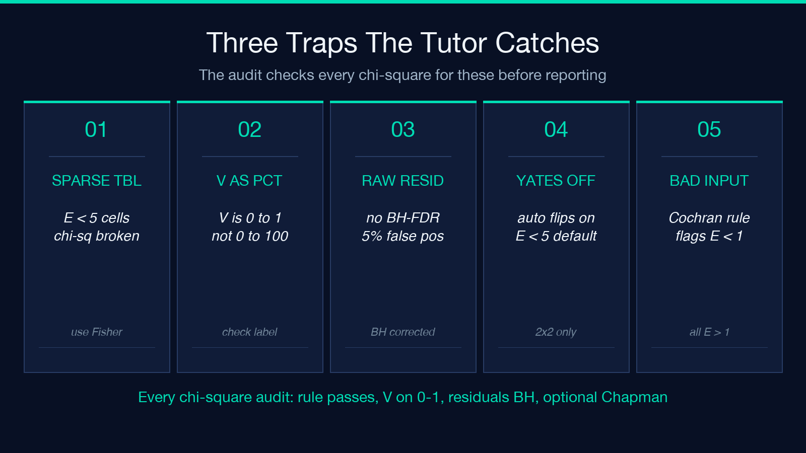
Trap 2 — Cramér’s V reported as a percentage. V ranges 0 to 1, not 0 to 100. If a result says “V = 23 percent” the author either multiplied by 100 or read a correlation coefficient. The tutor’s output panel labels it “Cramér’s V” with the raw value; check the number.
Trap 3 — raw residuals without multiplicity correction. A 10×10 table has 100 cells. Five percent exceeding 1.96 is expected by chance. Haberman adjusted + BH-FDR is the only way to know which cells are actually surprising. The tutor’s adjusted-residual panel with BH is the right unit of reporting; the raw residual column is for teaching.
When Cramér’s V Is the Whole Story
For survey research and A/B test reporting, the chi-square p-value answers “is there an association?” but the V answers “how big?”. A significant chi-square with V = 0.04 is statistically real and practically meaningless — 4 percent of the maximum explainable variance. Always pair the test statistic with the effect size; the tutor prints both on the same panel, so a single screenshot covers both columns of any results table.
When to Switch From Chi-Square to Logistic Regression
If your rows are ordinal (low / medium / high dose) or your cells have a natural ordering, the chi-square test of independence ignores the ordering and loses power. A logistic or ordinal regression on the same data respects the ordering and gives trend tests the chi-square cannot. The tutor is the right tool when the categories are nominal; reach for regression when they’re ordered.
Chapman Estimator — A 2×2 Specialty
Chapman (M+1)(C+1)/(R+1) - 1 estimates population size from a single mark-recapture pass where M is the number marked and released, C is the size of the second sample, R is the number recaptured. The +1 terms correct the Lincoln-Petersen bias for small samples. The tutor only emits Chapman when you enable the option because the formula looks identical to a 2×2 case-control odds ratio in shape, and they are not the same number.
Sample Configuration That Trips Everything
Paste "30, 20n20, 30". The 2×2 is balanced; expected counts are 25 per cell; chi-square = 4.0 (p = 0.0455); Yates = 3.24; G = 4.027; Cramér’s V = 0.2; adjusted residuals all equal ±2.0. Cochran’s rule passes — all E above 5, no sparsity. This is the textbook case where chi-square is fine, Fisher’s exact agrees, and the effect size is small but detectable. If you instead paste "5, 0n0, 5" (5 cells, 5 cells, with zeros), every expected count is 2.5 — Cochran trips, Fisher’s exact is the only reliable test, and the adjusted residual on the zero cells is the story. Run the live tutor with both inputs to see the difference.
What to Verify Before You Cite a Number
Four checks before any contingency table leaves your analysis. (1) Cochran’s rule passes, or you’re reporting Fisher’s exact. (2) Cramér’s V is on the 0-1 scale, not multiplied by 100. (3) Adjusted residuals are BH-corrected, not raw. (4) For mark-recapture data, you enabled the Chapman option. The tutor’s output panel satisfies all four when the configuration is right; the audit step is whether you read the warnings before reporting the headline. For worked examples across 2×2, 2×3, and 3×3 shapes, see the sibling A/B Test Significance Calculator and the ANOVA Analysis tool, which share the same expected-count and effect-size primitives for the categorical case. Explore more tools at elysiatools.com.
