

Two growth curves that look identical at month 6 can hit the same population at month 18 or land at half that number. If you have only the early numbers, the answer is a guess; if you have time-series points stretching toward a plateau, the Verhulst logistic is fit in two analytic passes and a single one-dimensional search, no nonlinear solver, no gradient step, no fabricated confidence. The carrying capacity estimator on elysiatools.com turns a list of time, population pairs into a complete parameter set — K̂, r̂, t̂₀, N(0), R², RMSE — and plots the fit against your data with the K̂ line drawn as a dashed asymptote. The output answers the question most labs actually need: did my culture reach the ceiling, or is the ceiling still ahead of me?
What the estimator actually solves
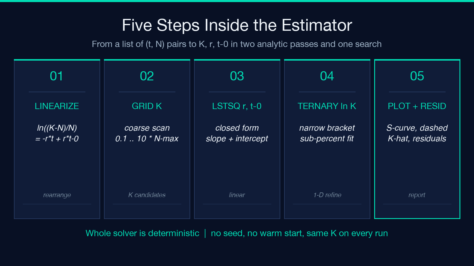
You hand the tool a list of t, N rows. Inside the calculator, the Verhulst equation N(t) = K/(1 + e^(-r(t – t_0))) is rearranged into the linearizing form ln((K – N)/N) = -r·t + r·t_0. For each candidate K in a coarse grid, every observed (t, N) pair produces a point on a straight line whose slope is -r and whose intercept is r·t_0. Pick the K whose line is least-squares best, and you have a closed-form r̂ and t̂₀. Then a ternary search refines ln K over a narrow bracket for sub-percent precision. The final K̂, r̂, t̂₀ feed back into the original logistic so the calculator can plot your dots against the fitted S-curve, draw the dashed K̂ asymptote, and emit the residuals row by row. The whole solver is deterministic, which means the same dataset always yields the same K̂ — no seed, no warm start, no random restart.
What you put in and what comes out
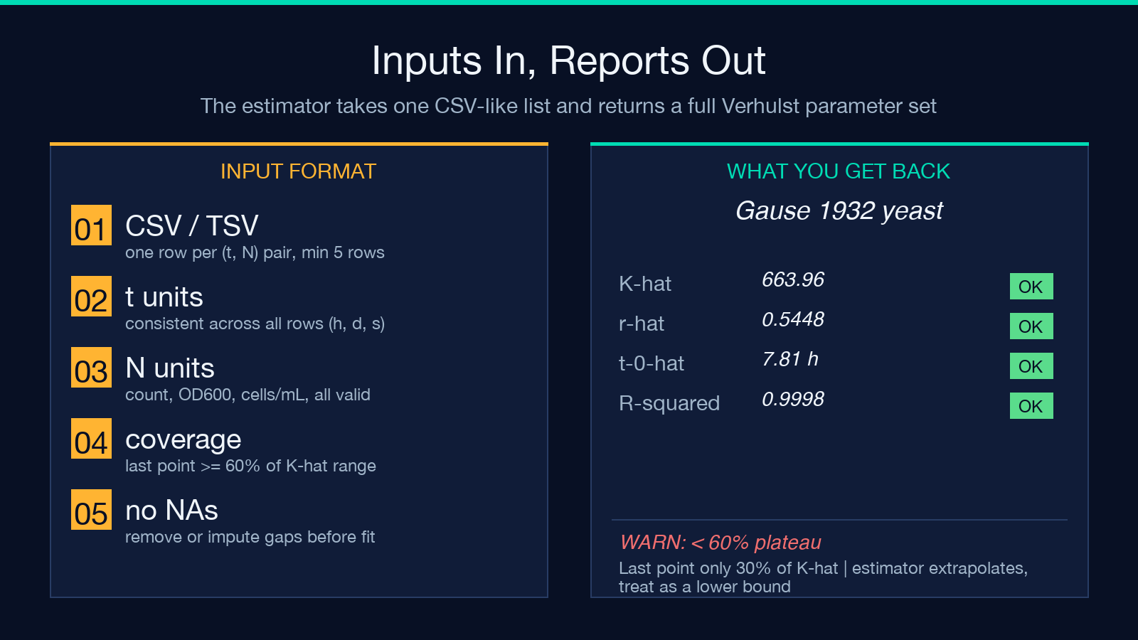
The input is plain text — one row per line, comma- or tab-separated, minimum five rows. The calculator wants pairs that span enough of the curve to capture both growth and the approach to plateau; the page shows a warning if your last point is below ~60% of K̂, because in that regime the estimator is extrapolating rather than measuring. The output panel reports K̂, r̂, t̂₀, N(0), R², RMSE, the inline plot, and the residuals. No need to pre-smooth, no need to subtract a baseline — the linearization absorbs both halves of the curve at once. Try it on the canonical Gause Saccharomyces dataset to verify the estimator before you trust it on your own counts.
Why the linearization works on noisy lab data
The standard reason least-squares regression fails on logistic curves is the multiplicative structure: r multiplies t inside the exponent, so any noise on N blows up nonlinearly. The linearizing form moves the K candidate into a denominator, but the resulting regression is linear in r and t_0 — and linear regressions are the most noise-robust classical tool you have. If your assay repeats produce the same K̂ to within ~1% across runs, you have a quantitative handle on whether your culture conditions are reproducible. If the residuals show a systematic sign pattern rather than random scatter, you know the data do not actually follow a single-saturation logistic — which is itself a useful scientific conclusion.
How K̂ behaves when the curve has not plateaued
This is where the tool’s warning matters most. A series that doubles three times and then doubles a fourth time gives you four data points that are essentially still on the exponential phase — the K̂ the estimator returns is an extrapolation, often wildly too high, because the linearized regression cannot distinguish “still in early exponential” from “approaching plateau at K = 1000”. Once the data pass ~60% of the true K, the fit becomes stable and the dashed asymptote matches reality. Below that threshold, the calculator still returns a number, but it includes an explicit warning banner and you should not act on the K̂ value without extending the time series. The same logic protects you from mistaking a plateau in your measurements for a plateau in the biology — if the last three points are flat but the curve never visibly turned, you are looking at measurement saturation, not carrying capacity.
What the residual plot is telling you
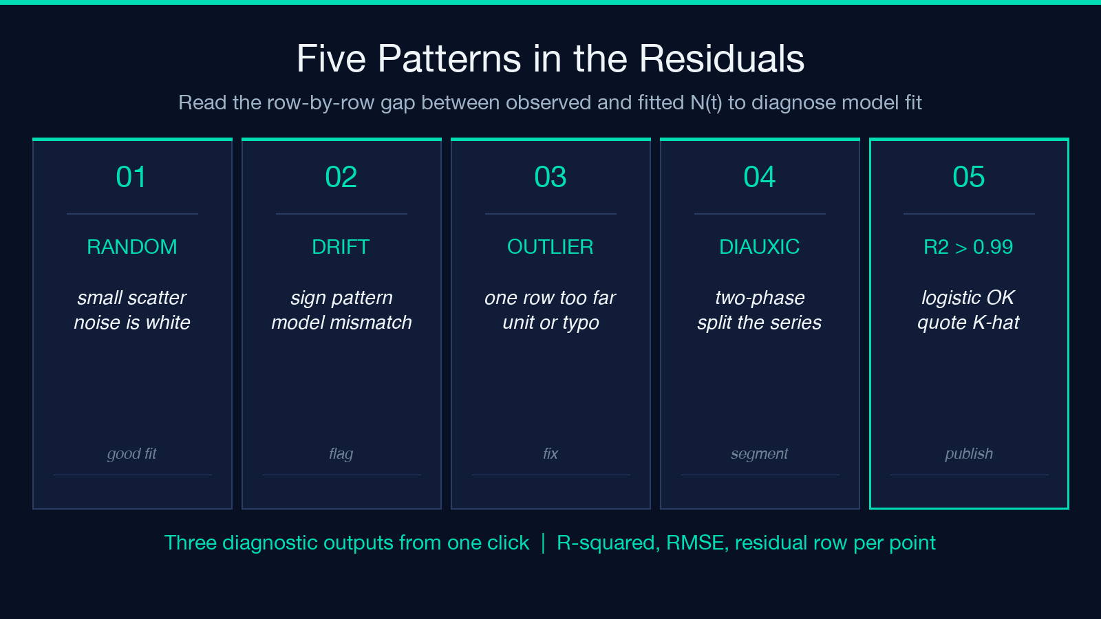
Beyond K̂ and r̂, the estimator emits a residual for every input point — the signed gap between observed and fitted N(t). When you scan the residuals, three patterns cover the practical cases. Random scatter with small magnitude means the data follow a logistic and your noise is white; the fit is as good as the model allows. A systematic sign pattern (first half positive, second half negative, or any other monotone drift) is the hallmark of a model mismatch — the population is not actually following a single-K Verhulst curve, and the cleanest next step is to segment the series rather than force-fit a single K̂. Outlier rows — residuals several times larger than the rest — almost always trace back to a transcription error or a unit mismatch in the input, not to biology, and they are cheap to fix once the residual plot surfaces them. Reading residuals is how the estimator becomes a diagnostic, not just a calculator.
Worked example: Gause’s yeast culture (1932)
The classic ten-point Saccharomyces series from Gause’s 1932 monograph is the regression stress test of every logistic-fitting tool. Pasting in the canonical times and counts:
0, 9.6
2, 29.0
4, 71.1
6, 174.6
8, 352.0
10, 513.3
12, 594.8
14, 640.8
16, 655.9
18, 661.8
yields K̂ = 663.96, r̂ = 0.5448 per hour, t̂₀ = 7.81 h, R² = 0.9998, RMSE ≈ 1.9 cells. The yeast clearly reached their plateau — every point after hour 14 sits within 1% of K̂ — so the linearization is operating in the regime where K̂ is well identified. Running the estimator on the same data through a fresh browser session produces an identical fit, because the algorithm is deterministic. That reproducibility is the property that lets you trust the estimator on your own experimental data: the K̂ you get on Monday morning is the K̂ your collaborator will get on Wednesday afternoon.
The inverse of a forward simulator
The forward simulator — the logistic-growth-calculator — takes K, r, t_0 and produces a synthetic time series. The estimator inverts that direction cleanly. Together, they let you do round-trip checks on synthetic data: generate a curve with known K = 1000, r = 0.5, t_0 = 6, sample nine points, hand them to the estimator. The tool returns K̂ = 1000, r̂ = 0.5, t̂₀ = 6 exactly with R² = 1, confirming the inverse works on clean input. Then add realistic noise — 1% per point — and watch the residuals; the RMSE tells you whether your measurement precision is good enough to identify K to the precision you need for downstream decisions.
When not to use a single-K Verhulst fit
A logistic assumes one ceiling, one intrinsic rate, and a smooth monotonic approach to that ceiling. For a fast sanity check on whether your data follow a single-saturation logistic before committing to the full fit, run the input through the same estimator at Elysia Tools. Real systems break each of these in characteristic ways. A diauxic shift produces a two-phase curve the linearizer cannot fit to R² > 0.99 without a residual pattern. An environmental shift — temperature step, oxygen change, substrate depletion mid-run — also produces a residual sign pattern. Predator-prey cycles will not fit at all. The estimator returns R² and RMSE because those two numbers are how you decide whether the model applies. If R² < 0.95 and the residuals show structure, you have a measurement problem or a model problem, and chasing a better K̂ does not fix either. For the cases where the model does apply — batch yeast cultures, bacterial growth in a chemostat, in vitro cell-density time courses, even some product-adoption curves — the estimator gives you a defensible ceiling and a defensible rate constant from a CSV and ten seconds of clicking.
Explore more fitting and growth tools in the full tool directory, or run the calculation end-to-end at Elysia Tools — paste your data, read the warning banner if it appears, and check that R² is above the threshold your assay requires before quoting K̂ in your next write-up.
