
Orifice flow is one of those calculations that looks elementary until the day the upstream pipe is sized wrong, the plate is bored at a beta ratio of 0.83, and the magmeter says 240 m³/h while the orifice meter claims 160. The Orifice Flow Calculator at Elysia Tools walks the four numbers that decide that disagreement — discharge coefficient, orifice diameter, differential pressure, fluid density — and reports volumetric flow, mass flow, and throat velocity in the same units your SCADA does.
What the ISO 5167 Bernoulli form actually computes
The thin-plate orifice is the oldest differential-pressure flow meter still in service. ISO 5167 collapses the bookkeeping into four measurable inputs and one empirical correction. Volumetric flow is Q = C_d · A · √(2·ΔP/ρ). Mass flow is ṁ = C_d · A · √(2·ρ·ΔP). Throat velocity is v_orifice = C_d · √(2·ΔP/ρ). Orifice area is A = π·d²/4, and from a supplied upstream pipe diameter D the calculator returns the diameter ratio β = d/D. The calculator accepts diameter in m / cm / mm, pressure in Pa / kPa / bar / atm / psi, and density in kg/m³ / g/cm³; output flow is reported in m³/s, L/s, L/min, and m³/h so a plant reading in gpm can compare without unit drift.
The Bernoulli form assumes incompressible flow. Gas service needs the compressibility expansion factor, which sits outside the thin-plate canonical form — that’s a Venturi or a V-Cone meter territory. The Orifice Flow Calculator is built for water, glycol mixes, light hydrocarbons, and any other liquid whose density stays within 1% across the plate.
What the discharge coefficient actually encodes
C_d is the single empirical term. ISO 5167 publishes tabulated values: 0.61 for a sharp-edged plate in the canonical tap configuration, rising to 0.62 for corner taps and approaching 0.66 for flange taps at low beta ratios. The coefficient folds in three losses — viscous drag through the bore, the vena contracta downstream of the plate, and the pressure-tap location. A technician who sets C_d = 1.0 because “Bernoulli is theoretical” is silently adding 60% more flow than the meter registers. A technician who copies 0.61 into every orifice regardless of beta ratio is reading the meter correctly at β = 0.5 and undercounting by 2-4% at β = 0.7. The calculator accepts C_d as a free input so a calibrated meter coefficient from the manufacturer’s nameplate can be entered directly. Elysia Tools defaults to 0.61 for the sharp-edged plate case.
Why the β-ratio sits between 0.2 and 0.7 in practice
β is the dimensionless ratio of orifice diameter to upstream pipe diameter. ISO 5167 calibrations are tabulated for 0.2 ≤ β ≤ 0.75. Below 0.2, the vena contracta sits far enough downstream that the corner-tap and D-tap pressure readings diverge; above 0.75, the plate approaches a nozzle-meter treatment and the empirical C_d shifts outside the calibrated band. Most plant piping lands at β = 0.5 because that ratio maximizes the differential pressure signal for a given line size — a 50 mm orifice in a 100 mm line, a 100 mm orifice in a 200 mm line — which is what the calculator’s worked example uses. Pushing β to 0.7 trades signal-to-noise (more ΔP, easier transmitter resolution) against pressure-recovery loss (more permanent head loss downstream).
A worked example: water at 100 kPa differential, 100 mm line
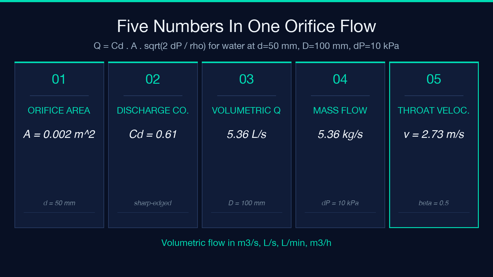
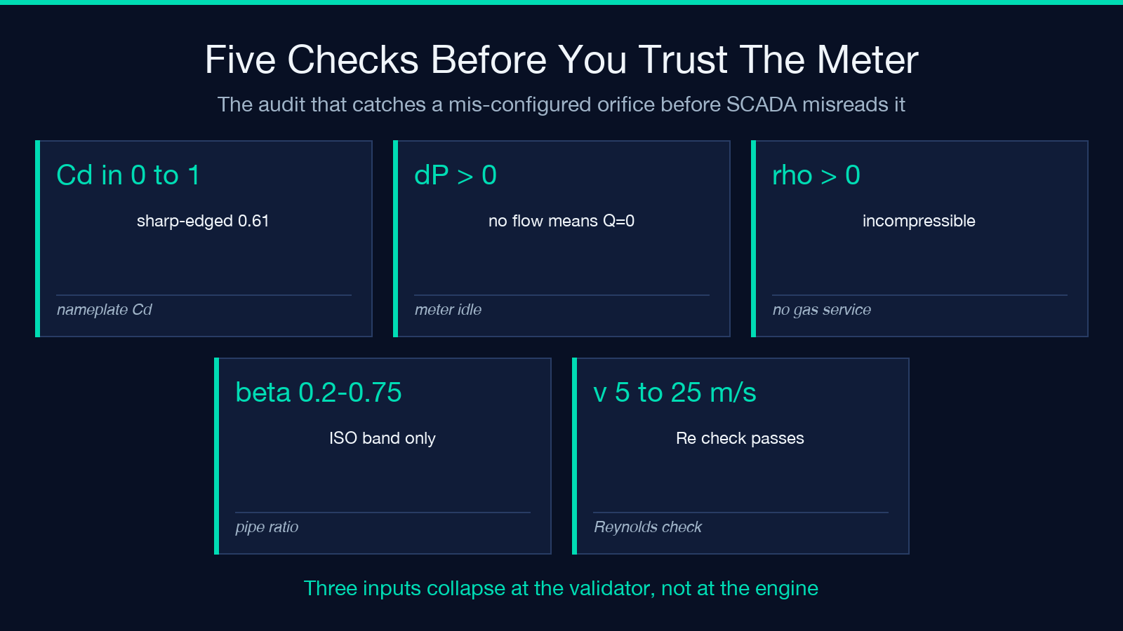
Set C_d = 0.61, d = 0.05 m, D = 0.1 m, ΔP = 10000 Pa, ρ = 1000 kg/m³. The orifice area is A = π·0.05²/4 = 0.0019635 m². The diameter ratio is β = 0.5. The square-root term is √(2·10000/1000) = √20 ≈ 4.472. Volumetric flow is Q = 0.61 · 0.0019635 · 4.472 ≈ 0.0054 m³/s — about 5.36 L/s, 321 L/min, or 19.3 m³/h. Mass flow is ṁ = 0.61 · 0.0019635 · √(2·1000·10000) ≈ 5.36 kg/s. Throat velocity is v = 0.61 · √20 ≈ 2.73 m/s. If the same orifice is dropped into a 150 mm line (β = 0.33) and the differential pressure rises to 25 kPa, the calculator will show Q ≈ 0.0067 m³/s — the meter is reading higher because ΔP is 2.5× larger even though the line is bigger. Open the Orifice Flow Calculator, enter the same five numbers, and the panel returns Q, ṁ, v_orifice, β, and A rounded to four decimal places in one pass.
Boundary cases that change the answer
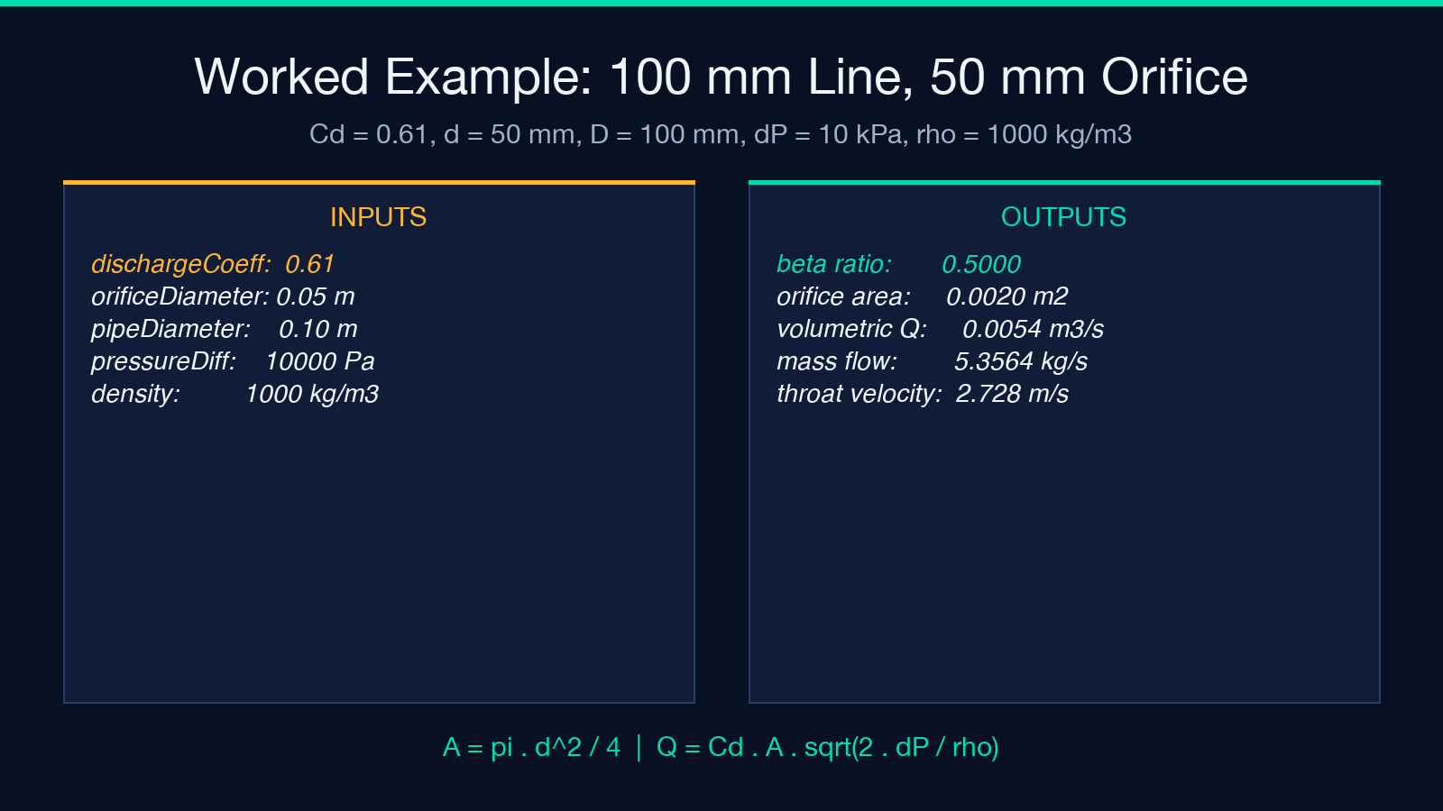
Three inputs collapse the formula. Setting ΔP = 0 returns Q = 0 regardless of the orifice size — a working meter with no flow correctly reports zero, not “leak through the plate.” Setting ρ = 0 returns a divide-by-zero because Bernoulli’s incompressible form requires a positive density. Setting C_d > 1 is a configuration error: discharge coefficients above 1.0 are physically impossible for a thin-plate orifice because the orifice restricts the flow path; a value above 1 indicates a misread nameplate or a confusion with the velocity-of-approach factor. The calculator refuses these inputs cleanly — the field is rejected at the validator, not silently rounded.
A subtler boundary case is gas service. Air at line pressure behaves compressibly: the expansion factor ε is below 1 and depends on the isentropic exponent, the pressure ratio ΔP/P₁, and the β-ratio. The thin-plate canonical form returns the incompressible estimate, which overstates gas flow by 5-15% at typical compressor-station differentials. For gas service, the Venturi meter (which uses the high-pressure-recovery geometry) is the more accurate instrument. The Orifice Flow Calculator is intentionally narrow — it does one form correctly rather than a family of forms approximately.
Verifying the meter reading with a side calculation
Three side-checks confirm the Bernoulli form is reading the meter correctly. First, dimensional consistency: A is in m², ΔP/ρ is in m²/s², √(ΔP/ρ) is in m/s, and the product is in m³/s — the units cancel. Second, throat velocity: v_orifice should land between 5 m/s and 25 m/s for a healthy liquid-service orifice; below 5 m/s, the Reynolds number is too low for the tabulated C_d; above 25 m/s, the permanent pressure loss becomes a significant fraction of the upstream pressure. Third, the Reynolds check: Re = ρ·v·D/μ should land above 10000 for the sharp-edged-plate C_d = 0.61 to hold. The calculator does not return Reynolds because μ is not an input, but the technician can compute it from v_orifice, D, and a viscosity lookup. When the orifice is reading correctly, all three checks agree within 2-3%.
Where orifice flow fits next to the other fluid-mechanics calculators
Orifice flow is one branch of differential-pressure flow metering. Sibling calculators on Elysia Tools cover the adjacent problems: the Bernoulli Equation Solver handles the free-form energy balance when there is no orifice plate and you need velocity from pressure drop or elevation; the Pipe Pressure Drop Calculator (Darcy-Weisbach) computes the line-side pressure loss that competes with the orifice’s own pressure recovery; the Pipe Friction Factor Calculator (Colebrook-White / Haaland) returns the Darcy friction factor f from Reynolds number and relative roughness, which feeds the line-side loss. Each tool shares the same engineering unit system; running all three on the same piping run shows whether the meter’s reading, the line’s loss, and the upstream pump’s head curve close into a consistent energy balance.
Closing
The Orifice Flow Calculator compresses a 100-year-old instrument formula into five inputs and four outputs, with the discharge coefficient and β-ratio sitting in the right places for ISO 5167 compliance. Drop the five numbers in, read Q, ṁ, v_orifice, β, and A in the units your plant uses, and the next disagreement between the orifice meter and the magmeter has somewhere to land that is not the SCADA engineer’s shift.
Explore more engineering calculators at elysiatools.com/en/tools.
